辐射神经场算法——Instant-NGP / Mipi-NeRF 360 / 3D Gaussian Splatting

辐射神经场算法——Instant-NGP / Mipi-NeRF 360 / 3D Gaussian Splatting

• 1. Instant-NGP
• • 1. MultiResolution Hash Encoding
  • 1.2 Accelerated Ray Marching
  • 1.3 实验结果
• 2. Mip-NeRF 360
• • 2.1 场景参数化
  • 2.2 在线蒸馏
  • 2.3 失真正则化
  • 2.4 实验结果
• 3. 3D Gaussian Splatting
• • 3.1 Differentiable 3D Gaussian Splatting
  • 3.2 Optimization with Adaptive Density Control of 3D Gaussians
  • 3.3 Fast Differentiable Rasterizer for Gaussians
  • 3.4 Spherical Harmonic(Supplement)
  • 3.5 实验结果

辐射神经场算法——NeRF算法详解
辐射神经场算法——Wild-NeRF / Mipi-NeRF / BARF / NSVF / Semantic-NeRF / DSNeRF
上面两篇博客是之前对NeRF相关算法的一些简单总结，离上一次工作中接触到NeRF相关的算法已经过去一年多的时间，最近大火的3D Gaussian Splatting让我忍不住想又跟进下这个方向的工作，我另外挑了两个比较有代表性的工作，一个是速度上SOAT的方法Instant-NGP，一个是效果上SOTA的方法Mipi NeRF 360，最后是3D Gaussian Splatting

1. Instant-NGP

Instant-NGP是2022年NVIDIA发布的一个项目，项目全称为《Instant Neural Graphics Primitives with a Multiresolution Hash Encoding》煤其主要贡献是通过Multiresolution Hash Encoding将NeRF的训练速度从小时级别缩短到秒级别。

在之前做NeRF加速的工作中，有一个经典的思路在所要表达的空间中构建Voxel，并在每个Voxel的节点上存储可训练的特征，在训练过程中同时更新MLP和Voxel节点特征，在推理过程中则使用先对Voxel节点特征进行插值，然后将插值后的特征再通过MLP进行推理。这样的好处可以使用更加局部的Voxel节点特征来表达空间，可以加速训练收敛，并且Voxel的分辨率越高，表达效果越好，但是模型占用的显存也越高，为此很多方法提出了Coarse-To-Fine的思路（例如NSVF和Plenoxels）或者Octree的数据结构（Plenoctree）来解决表达效果和显存占用的Trade Off问题，而本文提出的Multiresolution Hash Encoding也是为了解决该问题，但相对于前者，本文的方法更加优雅效果也更好，具体如下：

1. MultiResolution Hash Encoding

Multiresolution Hash Encoding的流程如下图所示：

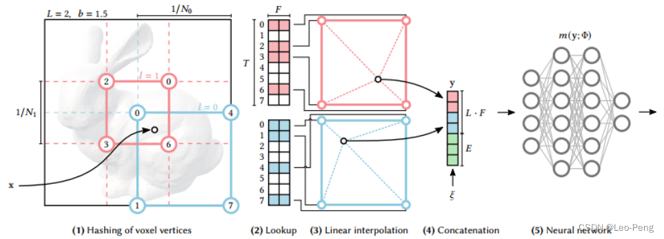
我们先定义一个$L$层分辨率的$d$维网格，在上图中$L$为2，$d$为2（在实际使用的Multiresolution Hash Encoding中$L$为16，$d$为3），分别由蓝色和红色表示，红色网格的分辨率为$1/N_0$（较低分辨率），蓝色网格的分辨率为$1/N_1$（较高分辨率），每个网格有四个顶点，那么每层网格的顶点数为$V={\left(N_l+1\right)}^d$。每层网格关联的特征向量个数为$T$，这个$T$是个超参，对于分辨率低的网格，顶点和特征向量是一对一的关系，但对于分辨率较高的网格，则会出现多个顶点对应同一个特征向量的情况，如果使用哈希表来记录这种对应关系的话，在高分辨率的网格中就会发生哈希碰撞。

具体步骤如下：

1. 对于给定的输入坐标$x$，我们在不同分辨率下找到对应的网格，即$x$落在$l_0$的右下网格，落在$l_1$的中间网格
2. 将网格的整数顶点映射成哈希表${\theta }_l$的索引值，通过该索引值直接索引到对应的特征向量，哈希表的大小为$T$，如果$V\le T$，则顶点和特征向量之间时$1:1$的映射，如果在分辨率更精细的网格中则$\mathrm{V}>\mathrm{T}$，此时就会出现哈希碰撞，但是在网络学习的过程中，越密集的区域对梯度影响越大，越稀疏的区域对梯度影响越小，网络会自动从密集区域提取样本，从而避免哈希碰撞
3. 从哈希表${\theta }_l$中找出四个索引值对应的特征向量后进行线性插值
4. 将不同分辨率网格插值后的特征向量以及辅助向量$\xi \in {\mathbb{R}}^E$进行Concat，然后输入MLP，后续操作和原始的NeRF就基本一致了

1.2 Accelerated Ray Marching

原始NeRF的射线采样算法是对射线进行均匀采样，采样过程分为粗采样和细采样，细采样根据粗采样的结果优化采样位置，在密度高的地方多采样，在密度低的地方少采样，但是在实际场景中，大多数是空白区域，固定采样策略会浪费大量资源。

Instant-NGP中射线采样采用的策略是离相机近的场景多采样，离相机远的场景少采样。并同时维护了一个根据场景大小变化并持续更新的占用栅格，通过Ray Matching过程中计算射线与占用栅格的交点，会主动跳过未被占用栅格中的采样。

1.3 实验结果

实验结果如下：

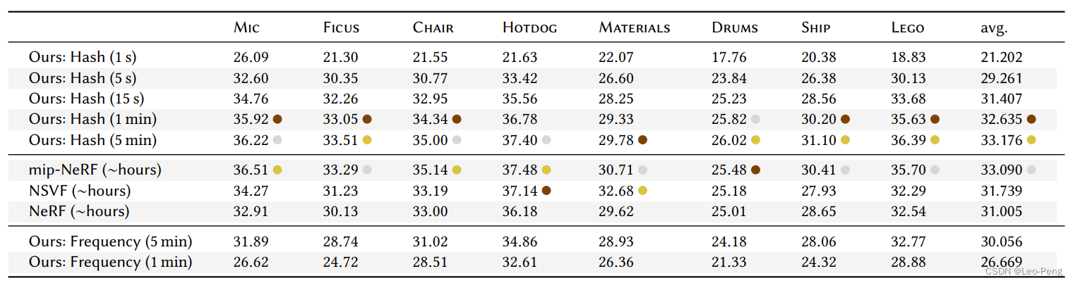
可以看到Instant-NGP在通过秒级别的训练就可以达到NeRF和NSVF通过若干个小时训练采可以达到的效果。

2. Mip-NeRF 360

Mip-NeRF 360的在NeRF++和Mip NeRF的基础上进行扩展，首先是整合了NeRF++提出的远景参数化技巧和Mip-NeRF的低通滤波思想，在此基础上扩展了场景参数化，在线蒸馏，失真正则化等方法来克服无界场景渲染中模糊和锯齿化等问题，均方误差较Mip-NeRF降低57%。

2.1 场景参数化

场景参数化解决无界场景中如何构建采样点的问题，在NeRF++中提出将无界场景分为前景和背景两部分分开渲染，前景在一个单位球体内使用正常的欧拉坐标系下的$(x,y,z)$表示采样点，背景使用一个四维向量$\left(x^{\prime },y^{\prime },z^{\prime },1/r\right)$表示，其中${\mathrm{x}}^{\prime 2}+{\mathrm{y}}^{\prime 2}+{\mathrm{z}}^{\prime 2}=1$表示方向，$0<1/r<1$表示方向，如下图所示：

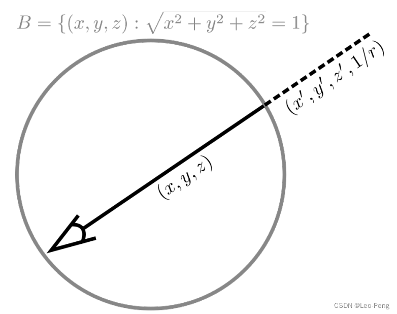
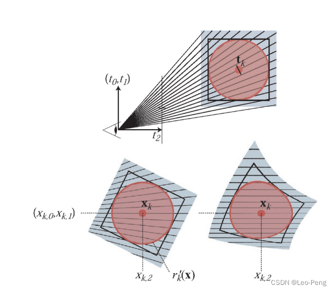
在Mip-NeRF 360中采用了类似的映射：$$\mathrm{contract}(\mathbf{x})=\{\begin{array}{ll}\mathbf{x}& \Vert \mathbf{x}\Vert \le 1\\ \left(2-\frac{1}{\Vert \mathbf{x}\Vert }\right)\left(\frac{\mathbf{x}}{\Vert \mathbf{x}\Vert }\right)& \Vert \mathbf{x}\Vert >1\end{array}$$但是由于Mip-NeRF中采样点不再只是一个点，而是通过一个3D高斯表达，因此当我们对背景采样点进行映射的时候，采样点对应的高斯方差也需要映射，这个过程有点像扩展卡尔曼滤波中的线性化状态转移部分，即$$f(\mathbf{x})\approx f(\mathbf{\mu })+{\mathbf{J}}_f(\mathbf{\mu })(\mathbf{x}-\mathbf{\mu })$$其中${\mathbf{J}}_f(\mathbf{\mu })$是映射方程$f(\mathbf{x})$相对于采样点$\mathbf{\mu }$的雅可比矩阵，然后高斯分布$(\mathbf{\mu },\mathbf{\Sigma })$就会被映射成$$f(\mathbf{\mu },\mathbf{\Sigma })=\left(f(\mathbf{\mu }),{\mathbf{J}}_f(\mathbf{\mu })\mathbf{\Sigma }{\mathbf{J}}_f(\mathbf{\mu }{)}^{\mathrm{T}}\right)$$下图就是Mip-NeRF中采样点的映射前后的示意图：

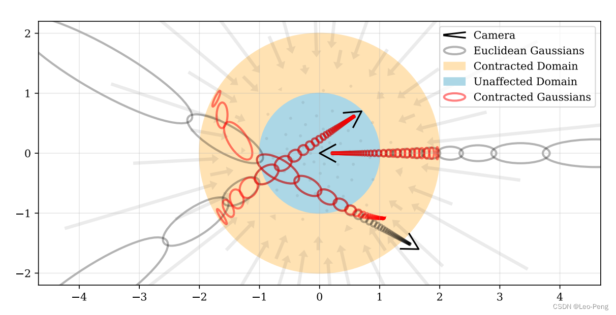
其中蓝色部分是欧式空间，黄色部分是非欧式空间，其中采样的坐标就是MLP的输入。在非欧式空间采样时，作者定义了一个从欧式空间射线距离$t$到非欧式空间距离$s$的可逆变换$$s\triangleq \frac{g(t)-g\left(t_n\right)}{g\left(t_f\right)-g\left(t_n\right)}$$$$t\triangleq g^{-1}\left(s\cdot g\left(t_f\right)+(1-s)\cdot g\left(t_n\right)\right)$$进一步作者定义了$g(x)=1/x$并在非欧式空间进行等距采样，这样就可以做满足在近处多采样，远处少采样的原则。

2.2 在线蒸馏

在原始NeRF中，使用了两个MLP分别作为Coarse和Fine两阶段训练，在Mip-NeRF中Coarse和Fine训练使用的是同一个MLP，在Mip-NeRF 360中作者对这一部分做了进一步优化，如下图所示：

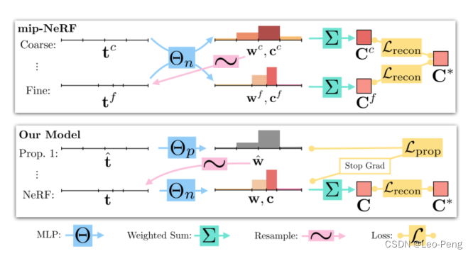
Mip-NeRF 360中使用了一个小的Proposal MLP和一个大的NeRF MLP，其中Proposal MLP仅输出密度用于指导重新采样的权重，在最后阶段使用NeRF MLP来渲染图像的颜色，这样的好处是可以减小计算量，但是没有直接的密度监督我们如何训练Proposal MLP呢？Mip-NeRF 360中使用了在线蒸馏的方式联合训练两个MLP

在线蒸馏的具体实现方式是通过损失函数${\mathcal{L}}_{\text{prop }}(\mathbf{t},\mathbf{w},\hat{\mathbf{t}},\hat{\mathbf{w}})$使得Proposal MLP的权重直方图$(\hat{\mathbf{t}},\hat{\mathbf{w}})$和NeRF MLP的权重直方图$(\mathbf{t},\mathbf{w})$保持一致，该函数定义如下：$${\mathcal{L}}_{\text{prop }}(\mathbf{t},\mathbf{w},\hat{\mathbf{t}},\hat{\mathbf{w}})=\sum \frac{1}{w}\max {\left(0,w_i-\mathrm{bound}\left(\hat{\mathbf{t}},\hat{\mathbf{w}},T_i\right)\right)}^2$$其中$$\mathrm{bound}(\hat{\mathbf{t}},\hat{\mathbf{w}},T)=\sum _{j:T\cap {\hat{T}}_j\ne \varnothing }{\hat{w}}_j$$bound $(\hat{\mathbf{t}},\hat{\mathbf{w}},T)$计算的是与区间$T$内所有Proposal权重的总和，该损失函数的含义是，如果两个直方图彼此一致，那么必须保持$w_i\le \mathrm{bound}\left(\hat{\mathbf{t}},\hat{\mathbf{w}},T_i\right)$，即保证两个直方图在相同区域的上界相同，又由于整个权重直方图的积分必须为1，因此两个直方图最终会趋于一致。

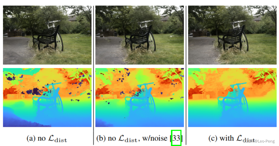
2.3 失真正则化

正则化的目的是消除一些深度不准确漂浮在前景中的背景点，解决方式是添加一个正则化损失：$${\mathcal{L}}_{\text{dist }}(\mathbf{s},\mathbf{w})={\int }_{-\infty }^{\infty }{\int }_{\mathbf{s}}{\mathbf{w}}_{\mathbf{s}}(u){\mathbf{w}}_{\mathbf{s}}(v)|u-v|d_u{d}_v$$其中$\mathbf{s}$为射线距离，$\mathbf{w}$为权重$${\mathbf{w}}_{\mathbf{s}}(u)=\sum _i{w}_i{1}_{\left[s_i,s_{i+1}\right)}(u)$$上述正则化损失的目标是使得单一射线上的权重分布更加接近于脉冲阶跃函数，离散化后，我们可以将损失函数写为$${\mathcal{L}}_{\text{dist }}(\mathbf{s},\mathbf{w})=\sum _{i,j}{w}_i{w}_j\left|\frac{s_i+s_{i+1}}{2}-\frac{s_j+s_{j+1}}{2}\right|+\frac{1}{3}\sum w_i^2\left(s_{i+1}-s_i\right)$$其中第一项最小化所有区间中点对之间的距离，使得区间越来越小，第二项最小化每个单独区间的加权大小，使得不同区间的权重越来越小，最后效果如下图所示：

2.4 实验结果

这里我们主要看下Ablation Study的结果：

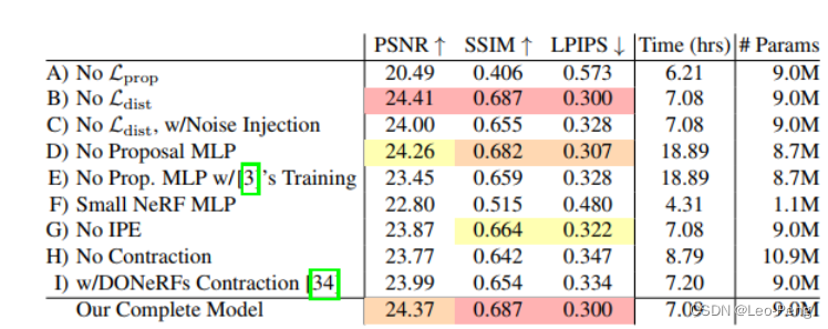
我们可以得到如下一些比较重要的结论：

1. 不使用${\mathcal{L}}_{\text{prop }}$，即不监督Proposal MLP会明显降低模型表现
2. 使用${\mathcal{L}}_{\text{dist }}$不会降低模型表现，并且可以减少不准确的背景深度
3. 使用Proposal MLP可以将训练速度加快3倍

3. 3D Gaussian Splatting

3D Gaussian Splatting的背景和重要性无需多言，以Instant-NGP的训练速度达到Mip-NeRF 360的渲染效果，下面我们结合源码来仔细读一读这篇Paper，在论文中提到，3D Gaussian Splatting有三个重要组件，分别是：

1. 引入3D高斯函数作为场景表达方法；
2. 在优化3D高斯函数属性的过程中，会添加和删除3D高斯函数实现自适应密度控制；
3. 实现针对GPU的快速、可微分的渲染方法；

下面我们从这三个方面展开下细节

3.1 Differentiable 3D Gaussian Splatting

我们简单复习下三维高斯函数的定义，一维高斯分布的概率密度函数为：$$p(x)=\frac{1}{\sigma \sqrt{2\pi }}\exp \left(-\frac{(x-\mu {)}^2}{2{\sigma }^2}\right)$$对于变量$\mathbf{v}=[a,b,c{]}^T$的三维高斯分布的概率密度函数如下：$$\begin{array}{rl}p(\mathbf{v})& =p(a)p(b)p(c)\\ & =\frac{1}{(2\pi {)}^{3/2}}\exp \left(-\frac{a^2+b^2+c^2}{2}\right)\\ & =\frac{1}{(2\pi {)}^{3/2}}\exp \left(-\frac{1}{2}{\mathbf{v}}^T\mathbf{v}\right)\\ & =\frac{1}{(2\pi {)}^{3/2}}\exp \left(-\frac{1}{2}(\mathbf{x}-\mu {)}^T{\mathbf{A}}^T\mathbf{A}(\mathbf{x}-\mu )\right)\end{array}$$其中定义$\mathbf{v}=\mathbf{A}(\mathbf{x}-\mu )$，其中$\mathbf{A}$为变换矩阵，则进一步变换为：$$p(\mathbf{v})=\frac{1}{(2\pi {)}^{3/2}}\exp \left(-\frac{1}{2}(\mathbf{x}-\mu {)}^T{\mathbf{A}}^T\mathbf{A}(\mathbf{x}-\mu )\right)$$对两边积分可以获得$$1={\iiint }_{-\infty }^{+\infty }\frac{1}{(2\pi {)}^{3/2}}\exp \left(-\frac{1}{2}(\mathbf{x}-\mu {)}^T{\mathbf{A}}^T\mathbf{A}(\mathbf{x}-\mu )\right)d\mathbf{v}$$其中$d\mathbf{v}=d(\mathbf{A}(\mathbf{x}-\mu ))=|\mathbf{A}|d\mathbf{x}$，则$$1={\iiint }_{-\infty }^{+\infty }\frac{|\mathbf{A}|}{(2\pi {)}^{3/2}}\exp \left(-\frac{1}{2}(\mathbf{x}-\mu {)}^T{\mathbf{A}}^T\mathbf{A}(\mathbf{x}-\mu )\right)d\mathbf{x}$$则三维高斯概率密度函数为$$p(\mathbf{x})=\frac{|\mathbf{A}|}{(2\pi {)}^{3/2}}\exp \left(-\frac{1}{2}(\mathbf{x}-\mu {)}^T{\mathbf{A}}^T\mathbf{A}(\mathbf{x}-\mu )\right)$$我们将变换矩阵$\mathbf{A}$转化为协方差矩阵$\mathbf{\Sigma }=\mathbf{A}{\mathbf{A}}^T$，则概率密度函数变为$$\begin{array}{rl}& p(\mathbf{x})=\frac{|\mathbf{A}|}{(2\pi {)}^{3/2}}\exp \left(-\frac{1}{2}(\mathbf{x}-\mu {)}^T{\mathbf{A}}^T\mathbf{A}(\mathbf{x}-\mu )\right)\\ & =\frac{1}{|\Sigma {|}^{1/2}(2\pi {)}^{3/2}}\exp \left(-\frac{1}{2}(\mathbf{x}-\mu {)}^T{\Sigma }^{-1}(\mathbf{x}-\mu )\right)\end{array}$$在3D Gaussian Splatting中正是使用这样一些具备3D高斯分布的点云来作为场景的表达，具体来说，包括：

1. 点的位置$\mathbf{x}$
2. 协方差矩阵$\Sigma$
3. 不透明度$\alpha$
4. 球谐函数稀疏（这个在下文3.4中单独补充相关知识）

这些也就是我们的优化变量，其中3D高斯函数定义为：$$G(x)=e^{-\frac{1}{2}(x{)}^T{\Sigma }^{-1}(x)}$$由于点的位置即高斯分布的均值以及没有积分为1的限制，因此我们可以忽略3D高斯概率密度函数中的均值和稀疏部分。

除了以上定义，还有三点需要我们注意：

1. 在实际渲染过程中，我们还需要将3D高斯分布投影到2D进行渲染，给定一个变换矩阵$W$，相机坐标下的协方差矩阵${\Sigma }^{\prime }$的定义为$${\Sigma }^{\prime }=JW\Sigma W^T{J}^T$$其中$J$为投影变换仿射近似的雅可比矩阵，这里为什么要做仿射近似呢？ 因为只有仿射变换才能保证三维的高斯分布投影到二维后仍然是一个高斯分布，也只有保持高斯分布我们才能对协方差进行分解和优化。我们定义相机投影公式为$\mathbf{x}=\varphi (\mathbf{t})$，其中$\mathbf{t}$为相机坐标系下3D点坐标，$\mathbf{x}$为投影到2D后的点坐标$$\left(\begin{array}{l}{x}_0\\ x_1\\ x_2\end{array}\right)=\varphi (\mathbf{t})=\left(\begin{array}{c}{t}_0/t_2\\ t_1/t_2\\ \Vert {\left(t_0,t_1,t_2\right)}^T\Vert \end{array}\right)$$$$\left(\begin{array}{l}{t}_0\\ t_1\\ t_2\end{array}\right)={\varphi }^{-1}(\mathbf{x})=\left(\begin{array}{c}{x}_0/l\cdot x_2\\ x_1/l\cdot x_2\\ 1/l\cdot x_2\end{array}\right)$$其中$l=\Vert {\left(x_0,x_1,1\right)}^T\Vert$，这个投影过程不具备仿射特性，如下右图所示，由于近大远小的原理，三维椭球体投影到二维图片上不一定是一个椭圆
   
   因此我们对投影公式$\varphi (\mathbf{t})$关于3D高斯分布的均值${\mathbf{t}}_k$求偏导$${\varphi }_k(\mathbf{t})={\mathbf{x}}_k+{\mathbf{J}}_k\cdot \left(\mathbf{t}-{\mathbf{t}}_k\right)$$其中$${\mathbf{J}}_k=\frac{\partial \varphi }{\partial \mathbf{t}}\left({\mathbf{t}}_k\right)=\left(\begin{array}{ccc}1/t_{k,2}& 0& -t_{k,0}/t_{k,2}^2\\ 0& 1/t_{k,2}& -t_{k,1}/t_{k,2}^2\\ t_{k,0}/l^{\prime }& t_{k,1}/l^{\prime }& t_{k,2}/l^{\prime }\end{array}\right)$$
   这部分代码可以参考：

__device__ float3 computeCov2D(const float3& mean, float focal_x, float focal_y, float tan_fovx, float tan_fovy, const float* cov3D, const float* viewmatrix) {     // The following models the steps outlined by equations 29     // and 31 in "EWA Splatting" (Zwicker et al., 2002).      // Additionally considers aspect / scaling of viewport.     // Transposes used to account for row-/column-major conventions.     // 将当前3D gaussian的中心点从世界坐标系投影到相机坐标系     float3 t = transformPoint4x3(mean, viewmatrix);      const float limx = 1.3f * tan_fovx;     const float limy = 1.3f * tan_fovy;     const float txtz = t.x / t.z;     const float tytz = t.y / t.z;     t.x = min(limx, max(-limx, txtz)) * t.z;     t.y = min(limy, max(-limy, tytz)) * t.z;      // 透视变换是非线性的，因为一个点的屏幕空间坐标与其深度（Z值）成非线性关系。雅可比矩阵 J 提供了一个在特定点附近的线性近似，这使得计算变得简单且高效     glm::mat3 J = glm::mat3(         focal_x / t.z, 0.0f, -(focal_x * t.x) / (t.z * t.z),         0.0f, focal_y / t.z, -(focal_y * t.y) / (t.z * t.z),         0, 0, 0);      glm::mat3 W = glm::mat3(         viewmatrix[0], viewmatrix[4], viewmatrix[8],         viewmatrix[1], viewmatrix[5], viewmatrix[9],         viewmatrix[2], viewmatrix[6], viewmatrix[10]);      glm::mat3 T = W * J;      glm::mat3 Vrk = glm::mat3(         cov3D[0], cov3D[1], cov3D[2],         cov3D[1], cov3D[3], cov3D[4],         cov3D[2], cov3D[4], cov3D[5]);      glm::mat3 cov = glm::transpose(T) * glm::transpose(Vrk) * T;      // Apply low-pass filter: every Gaussian should be at least     // one pixel wide/high. Discard 3rd row and column.     cov[0][0] += 0.3f;     cov[1][1] += 0.3f;     return { float(cov[0][0]), float(cov[0][1]), float(cov[1][1]) }; } 

2. 我们在优化的过程中，不能直接优化协方差矩阵$\Sigma$，原因是协方差矩阵$\Sigma$要求是半正定的，我们在梯度回传的过程中很难保证这一点，因此我们将协方差矩阵分解为缩放矩阵$S$和旋转矩阵$R$，即$$\Sigma =RS{S}^T{R}^T$$其中旋转矩阵$R$通过四元数$q$表示，缩放矩阵通过一个三维向量$s$表示，我们在优化过程中对四元数$q$进行归一化即可获得物理有效的单位四元数。
3. 在3D Gassian Splatting的代码实现中，训练过程没有使用自动微分，而是明确推导出了所有参数的梯度，推导过程如下：
   我们要计算的是相机坐标下的协方差矩阵${\Sigma }^{\prime }$相对四元数$q$和尺度向量$s$的雅可比：$$\frac{d{\Sigma }^{\prime }}{ds}=\frac{d{\Sigma }^{\prime }}{d\Sigma }\frac{d\Sigma }{ds}$$$$\frac{d{\Sigma }^{\prime }}{dq}=\frac{d{\Sigma }^{\prime }}{d\Sigma }\frac{d\Sigma }{dq}$$其中，${\Sigma }^{\prime }=JW\Sigma W^T{J}^T$，我们定义$U=JW$，而${\Sigma }^{\prime }$为$U\Sigma U^T$左上角$2\times 2$的矩阵（因为是平面投影的方差所以是二维的）$$\frac{\partial {\Sigma }^{\prime }}{\partial {\Sigma }_{ij}}=\left(\begin{array}{ll}{U}_{1,i}{U}_{1,j}& U_{1,i}{U}_{2,j}\\ U_{1,j}{U}_{2,i}& U_{2,i}{U}_{2,j}\end{array}\right)$$因为$\Sigma =RS{S}^T{R}^T$，定义$M=RS$则$\Sigma =M{M}^T$，那么有：$$\frac{d\Sigma }{ds}=\frac{d\Sigma }{dM}\frac{dM}{ds}$$$$\frac{d\Sigma }{dq}=\frac{d\Sigma }{dM}\frac{dM}{dq}$$其中$$\frac{d\Sigma }{dM}=2M^T$$$$\frac{\partial M_{i,j}}{\partial s_k}=\left\{\begin{array}{lr}{R}_{i,k}& \text{ if }\mathrm{j}=\mathrm{k}\\ 0& \text{ otherwise }\end{array}\right\}$$$$\frac{\partial M}{\partial q_r}=2\left(\begin{array}{ccc}0& -s_y{q}_k& s_z{q}_j\\ s_x{q}_k& 0& -s_z{q}_i\\ -s_x{q}_j& s_y{q}_i& 0\end{array}\right)$$$$\frac{\partial M}{\partial q_i}=2\left(\begin{array}{ccc}0& s_y{q}_j& s_z{q}_k\\ s_x{q}_j& -2s_y{q}_i& -s_z{q}_r\\ s_x{q}_k& s_y{q}_r& -2s_z{q}_i\end{array}\right)$$$$\frac{\partial M}{\partial q_j}=2\left(\begin{array}{ccc}-2s_x{q}_j& s_y{q}_i& s_z{q}_r\\ s_x{q}_i& 0& s_z{q}_k\\ -s_x{q}_r& s_y{q}_k& -2s_z{q}_j\end{array}\right)$$$$\frac{\partial M}{\partial q_k}=2\left(\begin{array}{ccc}-2s_x{q}_k& -s_y{q}_r& s_z{q}_i\\ s_x{q}_r& -2s_y{q}_k& s_z{q}_j\\ s_x{q}_i& s_y{q}_j& 0\end{array}\right)$$

3.2 Optimization with Adaptive Density Control of 3D Gaussians

3D Gaussian Splatting优化过程逻辑如下图所示：

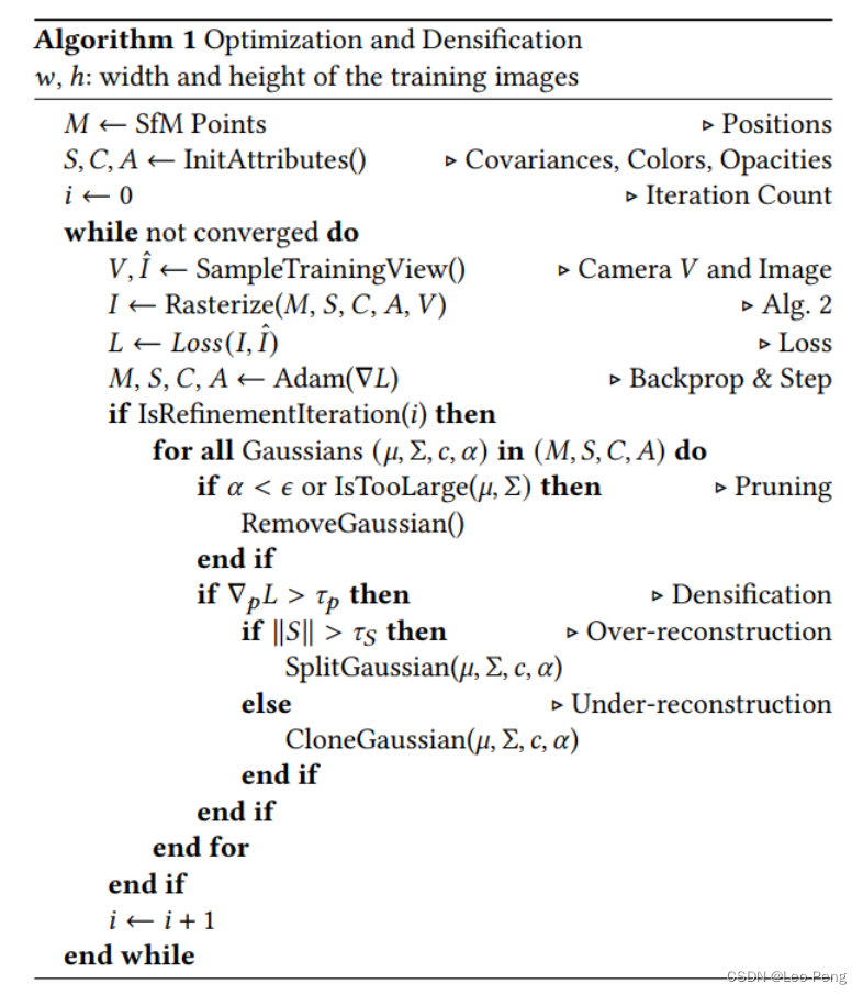
3D Gaussian从SFM输出的稀疏特征点进行初始化，在迭代过程中算法不断调整3D Gaussian的密度从而达到一个更密集的表示，从上面的伪代码中我们可以看到调整方式主要有如下三类：

1. 在重建不足的区域，如果小尺度的几何特征没有被足够覆盖，算法会克隆现有的高斯函数，即复制一个相同的高斯函数以增加局部密度，从而更好地捕捉细微的细节。
2. 对于过度重建的区域，如果小尺度的几何被一个大的高斯函数所覆盖，算法会将其分裂为两个较小的高斯函数，这样可以减少单一高斯函数覆盖过多细节的情况，避免模糊和不必要的重叠。
3. 每迭代一定次数就会删除基本透明的高斯函数，避免过多高斯函数对计算资源的消耗

这部分代码如下:

def densify_and_prune(self, max_grad, min_opacity, extent, max_screen_size):     grads = self.xyz_gradient_accum / self.denom             # 3Dgaussian的均值的累积梯度     grads[grads.isnan()] = 0.0      self.densify_and_clone(grads, max_grad, extent)          # 如果某些3Dgaussian的均值的梯度过大且尺度小于一定阈值，说明是欠重建，则对它们进行克隆     self.densify_and_split(grads, max_grad, extent)          # 如果某些3Dgaussian的均值的梯度过大且尺度超过一定阈值，说明是过重建，则对它们进行切分      prune_mask = (self.get_opacity < min_opacity).squeeze()  # 删除不透明度小于一定阈值的3Dgaussian     if max_screen_size:         big_points_vs = self.max_radii2D > max_screen_size   # 删除2D半径超过2D尺寸阈值的高斯         big_points_ws = self.get_scaling.max(dim=1).values > 0.1 * extent  # 删除尺度超过一定阈值的高斯         prune_mask = torch.logical_or(torch.logical_or(prune_mask, big_points_vs), big_points_ws)     self.prune_points(prune_mask)                            # 对不符合要求的高斯进行删除      torch.cuda.empty_cache()  def prune_points(self, mask):     valid_points_mask = ~mask     optimizable_tensors = self._prune_optimizer(valid_points_mask)      self._xyz = optimizable_tensors["xyz"]     self._features_dc = optimizable_tensors["f_dc"]     self._features_rest = optimizable_tensors["f_rest"]     self._opacity = optimizable_tensors["opacity"]     self._scaling = optimizable_tensors["scaling"]     self._rotation = optimizable_tensors["rotation"]      self.xyz_gradient_accum = self.xyz_gradient_accum[valid_points_mask]      self.denom = self.denom[valid_points_mask]     self.max_radii2D = self.max_radii2D[valid_points_mask]  # 删除不符合要求的3D gaussian在self.optimizer中对应的参数(均值、球谐系数、不透明度、尺度、旋转参数) def _prune_optimizer(self, mask):     optimizable_tensors = {}     for group in self.optimizer.param_groups:         stored_state = self.optimizer.state.get(group['params'][0], None)         if stored_state is not None:             stored_state["exp_avg"] = stored_state["exp_avg"][mask]             stored_state["exp_avg_sq"] = stored_state["exp_avg_sq"][mask]              del self.optimizer.state[group['params'][0]]             group["params"][0] = nn.Parameter((group["params"][0][mask].requires_grad_(True)))             self.optimizer.state[group['params'][0]] = stored_state              optimizable_tensors[group["name"]] = group["params"][0]         else:             group["params"][0] = nn.Parameter(group["params"][0][mask].requires_grad_(True))             optimizable_tensors[group["name"]] = group["params"][0]     return optimizable_tensors  # 对于那些均值的梯度超过一定阈值且尺度小于一定阈值的3D gaussian进行克隆操作 def densify_and_clone(self, grads, grad_threshold, scene_extent):     # Extract points that satisfy the gradient condition     selected_pts_mask = torch.where(torch.norm(grads, dim=-1) >= grad_threshold, True, False)     selected_pts_mask = torch.logical_and(selected_pts_mask,                                           torch.max(self.get_scaling, dim=1).values <= self.percent_dense*scene_extent)      new_xyz = self._xyz[selected_pts_mask]                         # (P, 3)     new_features_dc = self._features_dc[selected_pts_mask]         # (P, 1)     new_features_rest = self._features_rest[selected_pts_mask]     # (P, 15)     new_opacities = self._opacity[selected_pts_mask]               # (P, 1)     new_scaling = self._scaling[selected_pts_mask]                 # (P, 1)     new_rotation = self._rotation[selected_pts_mask]               # (P, 4)      self.densification_postfix(new_xyz, new_features_dc, new_features_rest, new_opacities, new_scaling, new_rotation)  # 对于那些均值的梯度超过一定阈值且尺度大于一定阈值的3D gaussian进行分割操作 def densify_and_split(self, grads, grad_threshold, scene_extent, N=2):     n_init_points = self.get_xyz.shape[0]     # Extract points that satisfy the gradient condition     padded_grad = torch.zeros((n_init_points), device="cuda")                      # (P,)     padded_grad[:grads.shape[0]] = grads.squeeze()     selected_pts_mask = torch.where(padded_grad >= grad_threshold, True, False)    # (P,)     selected_pts_mask = torch.logical_and(selected_pts_mask,                                           torch.max(self.get_scaling, dim=1).values > self.percent_dense*scene_extent)      stds = self.get_scaling[selected_pts_mask].repeat(N,1)                         # (2 * P, 3)     means = torch.zeros((stds.size(0), 3),device="cuda")                           # (2 * P, 3)     samples = torch.normal(mean=means, std=stds)                                   # (2 * P, 3)     rots = build_rotation(self._rotation[selected_pts_mask]).repeat(N,1,1)         # (2 * P, 3, 3)      # 在以原来3Dgaussian的均值xyz为中心, stds为形状, rots为方向的椭球内随机采样新的3Dgaussian     new_xyz = torch.bmm(rots, samples.unsqueeze(-1)).squeeze(-1) + self.get_xyz[selected_pts_mask].repeat(N, 1)  # (2 * P, 3)      # 由于原来的3D gaussian的尺度过大, 现在将3D gaussian的尺度缩小为原来的1/1.6     new_scaling = self.scaling_inverse_activation(self.get_scaling[selected_pts_mask].repeat(N,1) / (0.8*N))     # (2 * P, 3)     new_rotation = self._rotation[selected_pts_mask].repeat(N,1)                   # (2 * P, 4)     new_features_dc = self._features_dc[selected_pts_mask].repeat(N,1,1)           # (2 * P, 1, 3)     new_features_rest = self._features_rest[selected_pts_mask].repeat(N,1,1)       # (2 * P, 15, 3)     new_opacity = self._opacity[selected_pts_mask].repeat(N,1)                     # (2 * P, 1)      self.densification_postfix(new_xyz, new_features_dc, new_features_rest, new_opacity, new_scaling, new_rotation)      # 将原来的那些均值的梯度超过一定阈值且尺度大于一定阈值的3D gaussian进行删除 (因为已经将它们分割成了两个新的3D gaussian，原先的不再需要了)     prune_filter = torch.cat((selected_pts_mask, torch.zeros(N * selected_pts_mask.sum(), device="cuda", dtype=bool)))     self.prune_points(prune_filter)  # 将挑选出来的3D gaussian的参数拼接到原有的参数之后 def densification_postfix(self, new_xyz, new_features_dc, new_features_rest, new_opacities, new_scaling, new_rotation):     d = {"xyz": new_xyz,     "f_dc": new_features_dc,     "f_rest": new_features_rest,     "opacity": new_opacities,     "scaling" : new_scaling,     "rotation" : new_rotation}      optimizable_tensors = self.cat_tensors_to_optimizer(d)     self._xyz = optimizable_tensors["xyz"]     self._features_dc = optimizable_tensors["f_dc"]     self._features_rest = optimizable_tensors["f_rest"]     self._opacity = optimizable_tensors["opacity"]     self._scaling = optimizable_tensors["scaling"]     self._rotation = optimizable_tensors["rotation"]      self.xyz_gradient_accum = torch.zeros((self.get_xyz.shape[0], 1), device="cuda")     self.denom = torch.zeros((self.get_xyz.shape[0], 1), device="cuda")     self.max_radii2D = torch.zeros((self.get_xyz.shape[0]), device="cuda") 

3.3 Fast Differentiable Rasterizer for Gaussians

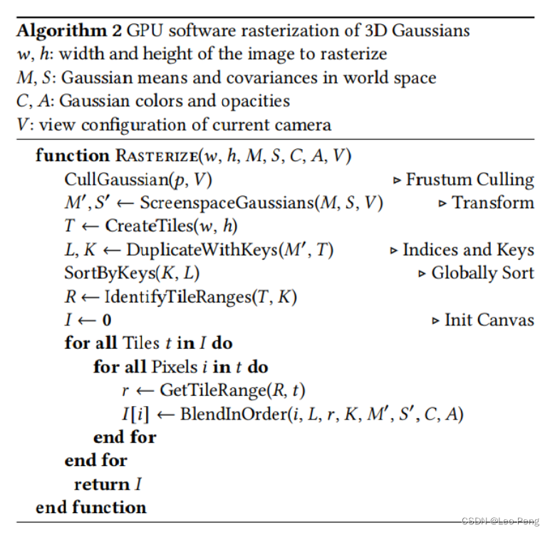
栅格化渲染流程如下图所示：

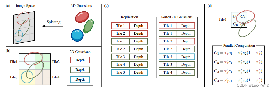
该过程又可以通过下图进行概括：

其主要步骤如下：

1. 首先将图片分割为$16\times 16$的Tile，保留与Tile构成的视锥的相较并且置信区间为99%的高斯函数；
2. 然后根据每个3D Gausssian相交的不同的Tile实例化不同的3D Gaussian对象，并为每个示例对象分配一个深度和Tile ID的键；
3. 根据这些键进行快速排序，排序后根据每个Tile中最近和最远的3D Gaussian对象，为每个Tile生成一个列表，然后每个Tile启动一个线程块，每个块首先将3D Gaussian对象加载到共享内存中，然后从前到后遍历列表来积累颜色和$\alpha$值，当$\alpha$值达到一定阈值时就停止渲染；

渲染过程分为前向和后向两部分，
其中前向过程如下：

int CudaRasterizer::Rasterizer::forward(     std::function<char* (size_t)> geometryBuffer,     std::function<char* (size_t)> binningBuffer,     std::function<char* (size_t)> imageBuffer,     const int P, int D, int M,     const float* background,     const int width, int height,     const float* means3D,     const float* shs,     const float* colors_precomp,     const float* opacities,     const float* scales,     const float scale_modifier,     const float* rotations,     const float* cov3D_precomp,     const float* viewmatrix,     const float* projmatrix,     const float* cam_pos,     const float tan_fovx, float tan_fovy,     const bool prefiltered,     float* out_color,     int* radii,     bool debug) {     const float focal_y = height / (2.0f * tan_fovy);   // 垂直方向的焦距 focal_y     const float focal_x = width / (2.0f * tan_fovx);    // 水平方向的焦距 focal_x      size_t chunk_size = required<GeometryState>(P);     // 计算存储所有3D gaussian的各个参数所需要的空间大小     char* chunkptr = geometryBuffer(chunk_size);        // 给所有3D gaussian的各个参数分配存储空间, 并返回存储空间的指针     GeometryState geomState = GeometryState::fromChunk(chunkptr, P);  // 在给定的内存块中初始化 GeometryState 结构体, 为不同成员分配空间，并返回一个初始化的实例      if (radii == nullptr)     {         radii = geomState.internal_radii;               // 指向radii数据的指针     }      // 定义了一个三维网格（dim3 是 CUDA 中定义三维网格维度的数据类型），确定了在水平和垂直方向上需要多少个块来覆盖整个渲染区域     dim3 tile_grid((width + BLOCK_X - 1) / BLOCK_X, (height + BLOCK_Y - 1) / BLOCK_Y, 1);     // 确定了每个块在 X（水平）和 Y（垂直）方向上的线程数     dim3 block(BLOCK_X, BLOCK_Y, 1);      // Dynamically resize image-based auxiliary buffers during training     size_t img_chunk_size = required<ImageState>(width * height);               // 计算存储所有2D pixel的各个参数所需要的空间大小     char* img_chunkptr = imageBuffer(img_chunk_size);                           // 给所有2D pixel的各个参数分配存储空间, 并返回存储空间的指针     ImageState imgState = ImageState::fromChunk(img_chunkptr, width * height);  // 在给定的内存块中初始化 ImageState 结构体, 为不同成员分配空间，并返回一个初始化的实例      if (NUM_CHANNELS != 3 && colors_precomp == nullptr)     {         throw std::runtime_error("For non-RGB, provide precomputed Gaussian colors!");     }      // Run preprocessing per-Gaussian (transformation, bounding, conversion of SHs to RGB)     CHECK_CUDA(FORWARD::preprocess(         P, D, M,                      // 3D gaussian的个数, 球谐函数的次数, 球谐系数的个数 (球谐系数用于表示颜色)         means3D,                      // 每个3D gaussian的XYZ均值         (glm::vec3*)scales,           // 每个3D gaussian的XYZ尺度         scale_modifier,               // 尺度缩放系数, 1.0         (glm::vec4*)rotations,        // 每个3D gaussian的旋转四元组         opacities,                    // 每个3D gaussian的不透明度         shs,                          // 每个3D gaussian的球谐系数, 用于表示颜色         geomState.clamped,            // 存储每个3D gaussian的R、G、B是否小于0         cov3D_precomp,                // 提前计算好的每个3D gaussian的协方差矩阵, []         colors_precomp,               // 提前计算好的每个3D gaussian的颜色, []         viewmatrix,                   // 相机外参矩阵, world to camera         projmatrix,                   // 投影矩阵, world to image         (glm::vec3*)cam_pos,          // 所有相机的中心点XYZ坐标         width, height,                // 图像的宽和高         focal_x, focal_y,             // 水平、垂直方向的焦距         tan_fovx, tan_fovy,           // 水平、垂直视场角一半的正切值         radii,                        // 存储每个2D gaussian在图像上的半径         geomState.means2D,            // 存储每个2D gaussian的均值         geomState.depths,             // 存储每个2D gaussian的深度         geomState.cov3D,              // 存储每个3D gaussian的协方差矩阵         geomState.rgb,                // 存储每个2D pixel的颜色         geomState.conic_opacity,      // 存储每个2D gaussian的协方差矩阵的逆矩阵以及它的不透明度         tile_grid,                    // 在水平和垂直方向上需要多少个块来覆盖整个渲染区域         geomState.tiles_touched,      // 存储每个2D gaussian覆盖了多少个tile         prefiltered                   // 是否预先过滤掉了中心点(均值XYZ)不在视锥（frustum）内的3D gaussian     ), debug)      // Compute prefix sum over full list of touched tile counts by Gaussians     // E.g., [2, 3, 0, 2, 1] -> [2, 5, 5, 7, 8]     CHECK_CUDA(cub::DeviceScan::InclusiveSum(geomState.scanning_space, geomState.scan_size, geomState.tiles_touched, geomState.point_offsets, P), debug)      // Retrieve total number of Gaussian instances to launch and resize aux buffers     int num_rendered;  // 存储所有的2D gaussian总共覆盖了多少个tile     // 将 geomState.point_offsets 数组中最后一个元素的值复制到主机内存中的变量 num_rendered     CHECK_CUDA(cudaMemcpy(&num_rendered, geomState.point_offsets + P - 1, sizeof(int), cudaMemcpyDeviceToHost), debug);      size_t binning_chunk_size = required<BinningState>(num_rendered);     char* binning_chunkptr = binningBuffer(binning_chunk_size);     BinningState binningState = BinningState::fromChunk(binning_chunkptr, num_rendered);      // 将每个3D gaussian的对应的tile index和深度存到point_list_keys_unsorted中     // 将每个3D gaussian的对应的index（第几个3D gaussian）存到point_list_unsorted中     // For each instance to be rendered, produce adequate [ tile | depth ] key      // and corresponding dublicated Gaussian indices to be sorted     duplicateWithKeys << <(P + 255) / 256, 256 >> > (         P,         geomState.means2D,         geomState.depths,         geomState.point_offsets,         binningState.point_list_keys_unsorted,         binningState.point_list_unsorted,         radii,         tile_grid)     CHECK_CUDA(, debug)      int bit = getHigherMsb(tile_grid.x * tile_grid.y);      // 对一个键值对列表进行排序。这里的键值对由 binningState.point_list_keys_unsorted 和 binningState.point_list_unsorted 组成     // 排序后的结果存储在 binningState.point_list_keys 和 binningState.point_list 中     // binningState.list_sorting_space 和 binningState.sorting_size 指定了排序操作所需的临时存储空间和其大小     // num_rendered 是要排序的元素总数。0, 32 + bit 指定了排序的最低位和最高位，这里用于确保排序考虑到了足够的位数，以便正确处理所有的键值对     // Sort complete list of (duplicated) Gaussian indices by keys     CHECK_CUDA(cub::DeviceRadixSort::SortPairs(         binningState.list_sorting_space,         binningState.sorting_size,         binningState.point_list_keys_unsorted, binningState.point_list_keys,         binningState.point_list_unsorted, binningState.point_list,         num_rendered, 0, 32 + bit), debug)      // 将 imgState.ranges 数组中的所有元素设置为 0     CHECK_CUDA(cudaMemset(imgState.ranges, 0, tile_grid.x * tile_grid.y * sizeof(uint2)), debug);      // 识别每个瓦片（tile）在排序后的高斯ID列表中的范围     // 目的是确定哪些高斯ID属于哪个瓦片，并记录每个瓦片的开始和结束位置     // Identify start and end of per-tile workloads in sorted list     if (num_rendered > 0)         identifyTileRanges << <(num_rendered + 255) / 256, 256 >> > (             num_rendered,             binningState.point_list_keys,             imgState.ranges);     CHECK_CUDA(, debug)      // Let each tile blend its range of Gaussians independently in parallel     const float* feature_ptr = colors_precomp != nullptr ? colors_precomp : geomState.rgb;     CHECK_CUDA(FORWARD::render(         tile_grid,                  // 在水平和垂直方向上需要多少个块来覆盖整个渲染区域         block,                      // 每个块在 X（水平）和 Y（垂直）方向上的线程数         imgState.ranges,            // 每个瓦片（tile）在排序后的高斯ID列表中的范围         binningState.point_list,    // 排序后的3D gaussian的id列表         width, height,              // 图像的宽和高         geomState.means2D,          // 每个2D gaussian在图像上的中心点位置         feature_ptr,                // 每个3D gaussian对应的RGB颜色         geomState.conic_opacity,    // 每个2D gaussian的协方差矩阵的逆矩阵以及它的不透明度         imgState.accum_alpha,       // 渲染过程后每个像素的最终透明度或透射率值         imgState.n_contrib,         // 每个pixel的最后一个贡献的2D gaussian是谁         background,                 // 背景颜色         out_color), debug)          // 输出图像      return num_rendered; } 

其中preprocess对应上图中( b )的流程，duplicateWithKeys和SortPairs对应上图中( c )的流程，render对应上图中( d )的流程
其中preprocess的代码如下，注意preprocess是对每个3D Gaussian进行并行的，输出的结果包括每个3D Gaussian的在2D上的协方差半径，位置，深度，颜色等用于后续的render：

void FORWARD::preprocess(int P, int D, int M,     const float* means3D,     const glm::vec3* scales,     const float scale_modifier,     const glm::vec4* rotations,     const float* opacities,     const float* shs,     bool* clamped,     const float* cov3D_precomp,     const float* colors_precomp,     const float* viewmatrix,     const float* projmatrix,     const glm::vec3* cam_pos,     const int W, int H,     const float focal_x, float focal_y,     const float tan_fovx, float tan_fovy,     int* radii,     float2* means2D,     float* depths,     float* cov3Ds,     float* rgb,     float4* conic_opacity,     const dim3 grid,     uint32_t* tiles_touched,     bool prefiltered) {     preprocessCUDA<NUM_CHANNELS> << <(P + 255) / 256, 256 >> > (         P, D, M,               // 3D gaussian的个数, 球谐函数的次数, 球谐系数的个数 (球谐系数用于表示颜色)         means3D,               // 每个3D gaussian的XYZ均值         scales,                // 每个3D gaussian的XYZ尺度         scale_modifier,        // 尺度缩放系数, 1.0         rotations,             // 每个3D gaussian的旋转四元组         opacities,             // 每个3D gaussian的不透明度         shs,                   // 每个3D gaussian的球谐系数, 用于表示颜色         clamped,               // 存储每个3D gaussian的R、G、B是否小于0         cov3D_precomp,         // 提前计算好的每个3D gaussian的协方差矩阵, []         colors_precomp,        // 提前计算好的每个3D gaussian的颜色, []         viewmatrix,            // 相机外参矩阵, world to camera         projmatrix,            // 投影矩阵, world to image         cam_pos,               // 所有相机的中心点XYZ坐标         W, H,                  // 图像的宽和高         tan_fovx, tan_fovy,    // 水平、垂直视场角一半的正切值         focal_x, focal_y,      // 水平、垂直方向的焦距         radii,                 // 存储每个2D gaussian在图像上的半径         means2D,               // 存储每个2D gaussian的均值         depths,                // 存储每个2D gaussian的深度         cov3Ds,                // 存储每个3D gaussian的协方差矩阵         rgb,                   // 存储每个2D pixel的颜色         conic_opacity,         // 存储每个2D gaussian的协方差矩阵的逆矩阵以及它的不透明度         grid,                  // 在水平和垂直方向上需要多少个tile来覆盖整个渲染区域         tiles_touched,         // 存储每个2D gaussian覆盖了多少个tile         prefiltered            // 是否预先过滤掉了中心点(均值XYZ)不在视锥（frustum）内的3D gaussian         ); }  // Perform initial steps for each Gaussian prior to rasterization. template<int C> __global__ void preprocessCUDA(int P, int D, int M,     const float* orig_points,     const glm::vec3* scales,     const float scale_modifier,     const glm::vec4* rotations,     const float* opacities,     const float* shs,     bool* clamped,     const float* cov3D_precomp,     const float* colors_precomp,     const float* viewmatrix,     const float* projmatrix,     const glm::vec3* cam_pos,     const int W, int H,     const float tan_fovx, float tan_fovy,     const float focal_x, float focal_y,     int* radii,     float2* points_xy_image,     float* depths,     float* cov3Ds,     float* rgb,     float4* conic_opacity,     const dim3 grid,     uint32_t* tiles_touched,     bool prefiltered) {     // 每个线程处理一个3D gaussian, index超过3D gaussian总数的线程直接返回, 防止数组越界访问     auto idx = cg::this_grid().thread_rank();     if (idx >= P)         return;      // Initialize radius and touched tiles to 0. If this isn't changed,     // this Gaussian will not be processed further.     radii[idx] = 0;     tiles_touched[idx] = 0;      // 判断当前处理的3D gaussian的中心点(均值XYZ)是否在视锥（frustum）内, 如果不在则直接返回     // Perform near culling, quit if outside.     float3 p_view;  // 用于存储将 p_orig 通过视图矩阵 viewmatrix 转换到视图空间后的点坐标     if (!in_frustum(idx, orig_points, viewmatrix, projmatrix, prefiltered, p_view))         return;      // Transform point by projecting     float3 p_orig = { orig_points[3 * idx], orig_points[3 * idx + 1], orig_points[3 * idx + 2] };     // 将当前3D gaussian的中心点从世界坐标系投影到裁剪坐标系     float4 p_hom = transformPoint4x4(p_orig, projmatrix);     float p_w = 1.0f / (p_hom.w + 0.0000001f);     // 将当前3D gaussian的中心点从裁剪坐标转变到归一化设备坐标（Normalized Device Coordinates, NDC）     float3 p_proj = { p_hom.x * p_w, p_hom.y * p_w, p_hom.z * p_w };      // If 3D covariance matrix is precomputed, use it, otherwise compute     // from scaling and rotation parameters.      const float* cov3D;     if (cov3D_precomp != nullptr)     {         cov3D = cov3D_precomp + idx * 6;     }     else     {         // 根据当前3D gaussian的尺度和旋转参数计算其对应的协方差矩阵         computeCov3D(scales[idx], scale_modifier, rotations[idx], cov3Ds + idx * 6);         cov3D = cov3Ds + idx * 6;     }      // 将当前的3D gaussian投影到2D图像，得到对应的2D gaussian的协方差矩阵cov     // Compute 2D screen-space covariance matrix     float3 cov = computeCov2D(p_orig, focal_x, focal_y, tan_fovx, tan_fovy, cov3D, viewmatrix);      // 计算当前2D gaussian的协方差矩阵cov的逆矩阵     // Invert covariance (EWA algorithm)     float det = (cov.x * cov.z - cov.y * cov.y);     if (det == 0.0f)         return;     float det_inv = 1.f / det;     float3 conic = { cov.z * det_inv, -cov.y * det_inv, cov.x * det_inv };      // 计算2D gaussian的协方差矩阵cov的特征值lambda1, lambda2, 从而计算2D gaussian的最大半径     // 对协方差矩阵进行特征值分解时，可以得到描述分布形状的主轴（特征向量）以及这些轴上分布的宽度（特征值）     // Compute extent in screen space (by finding eigenvalues of     // 2D covariance matrix). Use extent to compute a bounding rectangle     // of screen-space tiles that this Gaussian overlaps with. Quit if     // rectangle covers 0 tiles.      float mid = 0.5f * (cov.x + cov.z);     float lambda1 = mid + sqrt(max(0.1f, mid * mid - det));     float lambda2 = mid - sqrt(max(0.1f, mid * mid - det));     float my_radius = ceil(3.f * sqrt(max(lambda1, lambda2)));      // 将归一化设备坐标（Normalized Device Coordinates, NDC）转换为像素坐标     float2 point_image = { ndc2Pix(p_proj.x, W), ndc2Pix(p_proj.y, H) };     uint2 rect_min, rect_max;      // 计算当前的2D gaussian落在哪几个tile上     getRect(point_image, my_radius, rect_min, rect_max, grid);     // 如果没有命中任何一个title则直接返回     if ((rect_max.x - rect_min.x) * (rect_max.y - rect_min.y) == 0)         return;      // If colors have been precomputed, use them, otherwise convert     // spherical harmonics coefficients to RGB color.     if (colors_precomp == nullptr)     {         // 从每个3D gaussian对应的球谐系数中计算对应的颜色         glm::vec3 result = computeColorFromSH(idx, D, M, (glm::vec3*)orig_points, *cam_pos, shs, clamped);         rgb[idx * C + 0] = result.x;         rgb[idx * C + 1] = result.y;         rgb[idx * C + 2] = result.z;     }      // Store some useful helper data for the next steps.     depths[idx] = p_view.z;     radii[idx] = my_radius;     points_xy_image[idx] = point_image;     // Inverse 2D covariance and opacity neatly pack into one float4     conic_opacity[idx] = { conic.x, conic.y, conic.z, opacities[idx] };     tiles_touched[idx] = (rect_max.y - rect_min.y) * (rect_max.x - rect_min.x); } 

duplicateWithKeys代码如下，duplicateWithKeys同样是对每个3D Gaussian进行并行的，为每个3D Gaussian构建一个Key，根据这个Key进行排序就可以先按照Tile进行排序，再按照深度进行排序，这样就为每个Tile生成划分好了需要渲染的3D Gaussian对象。

__global__ void duplicateWithKeys(     int P,     const float2* points_xy,     const float* depths,     const uint32_t* offsets,     uint64_t* gaussian_keys_unsorted,     uint32_t* gaussian_values_unsorted,     int* radii,     dim3 grid) {     auto idx = cg::this_grid().thread_rank();     if (idx >= P)         return;      // Generate no key/value pair for invisible Gaussians     if (radii[idx] > 0)     {         // Find this Gaussian's offset in buffer for writing keys/values.         uint32_t off = (idx == 0) ? 0 : offsets[idx - 1];         uint2 rect_min, rect_max;          getRect(points_xy[idx], radii[idx], rect_min, rect_max, grid);          // For each tile that the bounding rect overlaps, emit a          // key/value pair. The key is |  tile ID  |      depth      |,         // and the value is the ID of the Gaussian. Sorting the values          // with this key yields Gaussian IDs in a list, such that they         // are first sorted by tile and then by depth.          for (int y = rect_min.y; y < rect_max.y; y++)         {             for (int x = rect_min.x; x < rect_max.x; x++)             {                 uint64_t key = y * grid.x + x;                 key <<= 32;                 key |= *((uint32_t*)&depths[idx]);                 gaussian_keys_unsorted[off] = key;                 gaussian_values_unsorted[off] = idx;                 off++;             }         }     } } 

render代码对应如下，在render函数中并行的方式是将每个Tile拆分为若干个Block，每个Block分配一个线程，每个线程处理Block中的一个像素，在每个线程中，每个像素会根据每个Tile关联的3D Gaussian循环处理获得最终的像素颜色：

void FORWARD::render(     const dim3 grid, dim3 block,     const uint2* ranges,     const uint32_t* point_list,     int W, int H,     const float2* means2D,     const float* colors,     const float4* conic_opacity,     float* final_T,     uint32_t* n_contrib,     const float* bg_color,     float* out_color) {     renderCUDA<NUM_CHANNELS> << <grid, block >> > (           ranges,             // 每个瓦片（tile）在排序后的高斯ID列表中的范围         point_list,         // 排序后的3D gaussian的id列表         W, H,               // 图像的宽和高         means2D,            // 每个2D gaussian在图像上的中心点位置         colors,             // 每个3D gaussian对应的RGB颜色         conic_opacity,      // 每个2D gaussian的协方差矩阵的逆矩阵以及它的不透明度         final_T,            // 渲染过程后每个像素的最终透明度或透射率值         n_contrib,          // 每个pixel的最后一个贡献的2D gaussian是谁         bg_color,           // 背景颜色         out_color);         // 输出图像 }   // Main rasterization method. Collaboratively works on one tile per // block, each thread treats one pixel. Alternates between fetching  // and rasterizing data. template <uint32_t CHANNELS> __global__ void __launch_bounds__(BLOCK_X * BLOCK_Y)  // 这是 CUDA 启动核函数时使用的线程格和线程块的数量 renderCUDA(     const uint2* __restrict__ ranges,     const uint32_t* __restrict__ point_list,     int W, int H,     const float2* __restrict__ points_xy_image,     const float* __restrict__ features,     const float4* __restrict__ conic_opacity,     float* __restrict__ final_T,     uint32_t* __restrict__ n_contrib,     const float* __restrict__ bg_color,     float* __restrict__ out_color) {     // Identify current tile and associated min/max pixel range.     auto block = cg::this_thread_block();     uint32_t horizontal_blocks = (W + BLOCK_X - 1) / BLOCK_X;     // 当前处理的tile的左上角的像素坐标     uint2 pix_min = { block.group_index().x * BLOCK_X, block.group_index().y * BLOCK_Y };     // 当前处理的tile的右下角的像素坐标     uint2 pix_max = { min(pix_min.x + BLOCK_X, W), min(pix_min.y + BLOCK_Y , H) };     // 当前处理的像素坐标     uint2 pix = { pix_min.x + block.thread_index().x, pix_min.y + block.thread_index().y };     // 当前处理的像素id     uint32_t pix_id = W * pix.y + pix.x;     // 当前处理的像素坐标     float2 pixf = { (float)pix.x, (float)pix.y };      // Check if this thread is associated with a valid pixel or outside.     bool inside = pix.x < W&& pix.y < H;     // Done threads can help with fetching, but don't rasterize     bool done = !inside;      // Load start/end range of IDs to process in bit sorted list.     // 当前处理的tile对应的3D gaussian的起始id和结束id     uint2 range = ranges[block.group_index().y * horizontal_blocks + block.group_index().x];     const int rounds = ((range.y - range.x + BLOCK_SIZE - 1) / BLOCK_SIZE);     // 还有多少3D gaussian需要处理     int toDo = range.y - range.x;      // Allocate storage for batches of collectively fetched data.     __shared__ int collected_id[BLOCK_SIZE];     __shared__ float2 collected_xy[BLOCK_SIZE];     __shared__ float4 collected_conic_opacity[BLOCK_SIZE];      // Initialize helper variables     float T = 1.0f;     uint32_t contributor = 0;     uint32_t last_contributor = 0;     float C[CHANNELS] = { 0 };      // Iterate over batches until all done or range is complete     for (int i = 0; i < rounds; i++, toDo -= BLOCK_SIZE)     {         // End if entire block votes that it is done rasterizing         int num_done = __syncthreads_count(done);         if (num_done == BLOCK_SIZE)             break;          // Collectively fetch per-Gaussian data from global to shared         int progress = i * BLOCK_SIZE + block.thread_rank();         if (range.x + progress < range.y)         {             // 当前处理的3D gaussian的id             int coll_id = point_list[range.x + progress];             collected_id[block.thread_rank()] = coll_id;             collected_xy[block.thread_rank()] = points_xy_image[coll_id];             collected_conic_opacity[block.thread_rank()] = conic_opacity[coll_id];         }         block.sync();          // Iterate over current batch         for (int j = 0; !done && j < min(BLOCK_SIZE, toDo); j++)         {             // Keep track of current position in range             contributor++;              // Resample using conic matrix (cf. "Surface              // Splatting" by Zwicker et al., 2001)             float2 xy = collected_xy[j];                     // 当前处理的2D gaussian在图像上的中心点坐标             float2 d = { xy.x - pixf.x, xy.y - pixf.y };     // 当前处理的2D gaussian的中心点到当前处理的pixel的offset             float4 con_o = collected_conic_opacity[j];       // 当前处理的2D gaussian的协方差矩阵的逆矩阵以及它的不透明度             // 计算高斯分布的强度（或权重），用于确定像素在光栅化过程中的贡献程度             float power = -0.5f * (con_o.x * d.x * d.x + con_o.z * d.y * d.y) - con_o.y * d.x * d.y;             if (power > 0.0f)                 continue;              // Eq. (2) from 3D Gaussian splatting paper.             // Obtain alpha by multiplying with Gaussian opacity             // and its exponential falloff from mean.             // Avoid numerical instabilities (see paper appendix).              float alpha = min(0.99f, con_o.w * exp(power));             if (alpha < 1.0f / 255.0f)                 continue;             float test_T = T * (1 - alpha);             if (test_T < 0.0001f)             {                 done = true;                 continue;             }              // Eq. (3) from 3D Gaussian splatting paper.             for (int ch = 0; ch < CHANNELS; ch++)                 C[ch] += features[collected_id[j] * CHANNELS + ch] * alpha * T;              T = test_T;              // Keep track of last range entry to update this             // pixel.             last_contributor = contributor;         }     }      // All threads that treat valid pixel write out their final     // rendering data to the frame and auxiliary buffers.     if (inside)     {         final_T[pix_id] = T;                     // 渲染过程后每个像素的最终透明度或透射率值         n_contrib[pix_id] = last_contributor;    // 最后一个贡献的2D gaussian是谁         for (int ch = 0; ch < CHANNELS; ch++)             out_color[ch * H * W + pix_id] = C[ch] + T * bg_color[ch];     } } 

反向过程我们主要看下render函数，在论文中作者有提到：

during the backward pass, we must therefore recover the full sequence of blended points per-pixel in the forward pass. One solution would be to store arbitrarily long lists of blended points per-pixel in global memory [Kopanas et al. 2021]. To avoid the implied dynamic memory management overhead, we instead choose to traverse the pertile lists again; we can reuse the sorted array of Gaussians and tile ranges from the forward pass

从代码中我们可以看到，在反向传播的过程中算法重新计算了每个Block的信息，同时使用到了前向传播中记录的final_Ts和n_contrib来辅助进行梯度回传。

void BACKWARD::render(     const dim3 grid, const dim3 block,     const uint2* ranges,     const uint32_t* point_list,     int W, int H,     const float* bg_color,     const float2* means2D,     const float4* conic_opacity,     const float* colors,     const float* final_Ts,     const uint32_t* n_contrib,     const float* dL_dpixels,     float3* dL_dmean2D,     float4* dL_dconic2D,     float* dL_dopacity,     float* dL_dcolors) {     renderCUDA<NUM_CHANNELS> << <grid, block >> >(         ranges,         point_list,         W, H,         bg_color,         means2D,         conic_opacity,         colors,         final_Ts,         n_contrib,         dL_dpixels,         dL_dmean2D,         dL_dconic2D,         dL_dopacity,         dL_dcolors         ); }  // Backward version of the rendering procedure. template <uint32_t C> __global__ void __launch_bounds__(BLOCK_X * BLOCK_Y) renderCUDA(     const uint2* __restrict__ ranges,     const uint32_t* __restrict__ point_list,     int W, int H,     const float* __restrict__ bg_color,     const float2* __restrict__ points_xy_image,     const float4* __restrict__ conic_opacity,     const float* __restrict__ colors,     const float* __restrict__ final_Ts,     const uint32_t* __restrict__ n_contrib,     const float* __restrict__ dL_dpixels,     float3* __restrict__ dL_dmean2D,     float4* __restrict__ dL_dconic2D,     float* __restrict__ dL_dopacity,     float* __restrict__ dL_dcolors) {     // We rasterize again. Compute necessary block info.     auto block = cg::this_thread_block();     const uint32_t horizontal_blocks = (W + BLOCK_X - 1) / BLOCK_X;     const uint2 pix_min = { block.group_index().x * BLOCK_X, block.group_index().y * BLOCK_Y };     const uint2 pix_max = { min(pix_min.x + BLOCK_X, W), min(pix_min.y + BLOCK_Y , H) };     const uint2 pix = { pix_min.x + block.thread_index().x, pix_min.y + block.thread_index().y };     const uint32_t pix_id = W * pix.y + pix.x;     const float2 pixf = { (float)pix.x, (float)pix.y };      const bool inside = pix.x < W&& pix.y < H;     // 当前处理的tile对应的3D gaussian的起始id和结束id     const uint2 range = ranges[block.group_index().y * horizontal_blocks + block.group_index().x];     const int rounds = ((range.y - range.x + BLOCK_SIZE - 1) / BLOCK_SIZE);      bool done = !inside;     int toDo = range.y - range.x;      __shared__ int collected_id[BLOCK_SIZE];     __shared__ float2 collected_xy[BLOCK_SIZE];     __shared__ float4 collected_conic_opacity[BLOCK_SIZE];     __shared__ float collected_colors[C * BLOCK_SIZE];      // In the forward, we stored the final value for T, the     // product of all (1 - alpha) factors.      const float T_final = inside ? final_Ts[pix_id] : 0;     float T = T_final;      // We start from the back. The ID of the last contributing     // Gaussian is known from each pixel from the forward.     uint32_t contributor = toDo;     const int last_contributor = inside ? n_contrib[pix_id] : 0;      float accum_rec[C] = { 0 };     float dL_dpixel[C];         // 当前pixel对应的梯度     if (inside)         for (int i = 0; i < C; i++)             dL_dpixel[i] = dL_dpixels[i * H * W + pix_id];      float last_alpha = 0;     float last_color[C] = { 0 };      // Gradient of pixel coordinate w.r.t. normalized      // screen-space viewport corrdinates (-1 to 1)     const float ddelx_dx = 0.5 * W;     const float ddely_dy = 0.5 * H;      // Traverse all Gaussians     for (int i = 0; i < rounds; i++, toDo -= BLOCK_SIZE)     {         // Load auxiliary data into shared memory, start in the BACK         // and load them in revers order.         block.sync();         const int progress = i * BLOCK_SIZE + block.thread_rank();         if (range.x + progress < range.y)         {             const int coll_id = point_list[range.y - progress - 1];             collected_id[block.thread_rank()] = coll_id;             collected_xy[block.thread_rank()] = points_xy_image[coll_id];             collected_conic_opacity[block.thread_rank()] = conic_opacity[coll_id];             for (int i = 0; i < C; i++)                 collected_colors[i * BLOCK_SIZE + block.thread_rank()] = colors[coll_id * C + i];         }         block.sync();          // Iterate over Gaussians         for (int j = 0; !done && j < min(BLOCK_SIZE, toDo); j++)         {             // Keep track of current Gaussian ID. Skip, if this one             // is behind the last contributor for this pixel.             contributor--;             if (contributor >= last_contributor)                 continue;              // Compute blending values, as before.             const float2 xy = collected_xy[j];             const float2 d = { xy.x - pixf.x, xy.y - pixf.y };             const float4 con_o = collected_conic_opacity[j];             const float power = -0.5f * (con_o.x * d.x * d.x + con_o.z * d.y * d.y) - con_o.y * d.x * d.y;             if (power > 0.0f)                 continue;              const float G = exp(power);             const float alpha = min(0.99f, con_o.w * G);             if (alpha < 1.0f / 255.0f)                 continue;              T = T / (1.f - alpha);             const float dchannel_dcolor = alpha * T;              // Propagate gradients to per-Gaussian colors and keep             // gradients w.r.t. alpha (blending factor for a Gaussian/pixel             // pair).             float dL_dalpha = 0.0f;             const int global_id = collected_id[j];             for (int ch = 0; ch < C; ch++)             {                 const float c = collected_colors[ch * BLOCK_SIZE + j];                 // Update last color (to be used in the next iteration)                 accum_rec[ch] = last_alpha * last_color[ch] + (1.f - last_alpha) * accum_rec[ch];                 last_color[ch] = c;                  const float dL_dchannel = dL_dpixel[ch];                 dL_dalpha += (c - accum_rec[ch]) * dL_dchannel;                 // Update the gradients w.r.t. color of the Gaussian.                  // Atomic, since this pixel is just one of potentially                 // many that were affected by this Gaussian.                 atomicAdd(&(dL_dcolors[global_id * C + ch]), dchannel_dcolor * dL_dchannel);             }             dL_dalpha *= T;             // Update last alpha (to be used in the next iteration)             last_alpha = alpha;              // Account for fact that alpha also influences how much of             // the background color is added if nothing left to blend             float bg_dot_dpixel = 0;             for (int i = 0; i < C; i++)                 bg_dot_dpixel += bg_color[i] * dL_dpixel[i];             dL_dalpha += (-T_final / (1.f - alpha)) * bg_dot_dpixel;              // Helpful reusable temporary variables             const float dL_dG = con_o.w * dL_dalpha;             const float gdx = G * d.x;             const float gdy = G * d.y;             const float dG_ddelx = -gdx * con_o.x - gdy * con_o.y;             const float dG_ddely = -gdy * con_o.z - gdx * con_o.y;              // Update gradients w.r.t. 2D mean position of the Gaussian             atomicAdd(&dL_dmean2D[global_id].x, dL_dG * dG_ddelx * ddelx_dx);             atomicAdd(&dL_dmean2D[global_id].y, dL_dG * dG_ddely * ddely_dy);              // Update gradients w.r.t. 2D covariance (2x2 matrix, symmetric)             atomicAdd(&dL_dconic2D[global_id].x, -0.5f * gdx * d.x * dL_dG);             atomicAdd(&dL_dconic2D[global_id].y, -0.5f * gdx * d.y * dL_dG);             atomicAdd(&dL_dconic2D[global_id].w, -0.5f * gdy * d.y * dL_dG);              // Update gradients w.r.t. opacity of the Gaussian             atomicAdd(&(dL_dopacity[global_id]), G * dL_dalpha);         }     } } 

3.4 Spherical Harmonic(Supplement)

我知道的最先将球谐函数引入NeRF的相关工作是PlenOctree，后续高效渲染的方法Plenonxels中也用到了球谐函数，这里我们对球谐函数的基本知识做一个简单介绍

球谐函数是在球面坐标系下的一种基函数，球谐函数的公式：$$Y_{\ell }^m(\theta ,\varphi )=\sqrt{\frac{2\ell +1}{4\pi }\frac{(\ell -m)!}{(\ell +m)!}}{P}_{\ell }^m(\cos \theta )e^{im\varphi }$$其中输入是两个角度值$\theta$和$\varphi$，参数$l$和$m$定义了不同阶的球谐函数，如下就是不同阶球谐函数的可视化结果，从上到下分别是$l=0$到$l=3$，从做到右分别是$m=-l$和$m=l$：

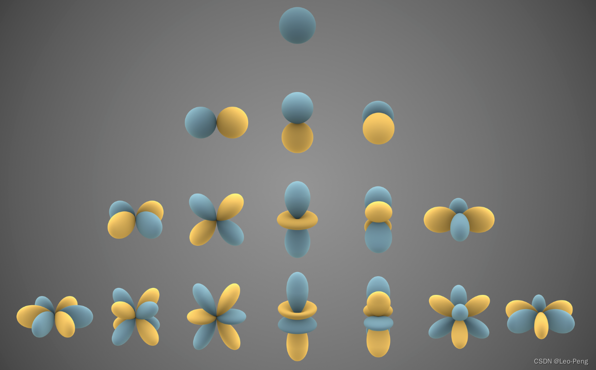
有了这些基函数，我们就可以将任意一个球面坐标系下的表达进行分解$$C(\theta ,\varphi )=\sum _{j=0}^J\sum _{m=-j}^j{c}_j^m{Y}_j^m(\theta ,\varphi )$$其中$c$代表球谐系数，这个过程类似于傅里叶展开，只不过傅里叶展开是在笛卡尔坐标系下使用三角函数作为基函数对目标函数进行分解。

那么我们为什么要使用球谐函数呢？在原始的NeRF中，我们对输入位置和角度都会加入Positional Encoding：$$\gamma (p)=\left(\sin \left(2^0\pi p\right),\cos \left(2^0\pi p\right),\cdots ,\sin \left(2^{L-1}\pi p\right),\cos \left(2^{L-1}\pi p\right)\right)$$上述Positional Encoding是一种频率编码，是一种广义的傅里叶变换，在笛卡尔坐标系下可以使用三角函数作为基函数进行傅里叶变换是合理的，但是角度值$\theta$和$\varphi$其实是建立在球面坐标系下，因此使用球谐函数作为基函数会更加合理

使用球谐函数有什么收益呢？在PlenOctree的论文中有对比使用球谐函数后训练速度加快了约10%但渲染效果没有明显差异，在使用细节上，球谐函数使用到3阶即可达到比较不错的效果，更高的阶数会映入更多的参数，但是效果提升却变得有限。

这部分代码如下：

// 从每个3D gaussian对应的球谐系数中计算对应的颜色 // Forward method for converting the input spherical harmonics // coefficients of each Gaussian to a simple RGB color. __device__ glm::vec3 computeColorFromSH(int idx, int deg, int max_coeffs, const glm::vec3* means, glm::vec3 campos, const float* shs, bool* clamped) {     // The implementation is loosely based on code for      // "Differentiable Point-Based Radiance Fields for      // Efficient View Synthesis" by Zhang et al. (2022)     glm::vec3 pos = means[idx];     glm::vec3 dir = pos - campos;     dir = dir / glm::length(dir);      glm::vec3* sh = ((glm::vec3*)shs) + idx * max_coeffs;     glm::vec3 result = SH_C0 * sh[0];      if (deg > 0)     {         float x = dir.x;         float y = dir.y;         float z = dir.z;         result = result - SH_C1 * y * sh[1] + SH_C1 * z * sh[2] - SH_C1 * x * sh[3];          if (deg > 1)         {             float xx = x * x, yy = y * y, zz = z * z;             float xy = x * y, yz = y * z, xz = x * z;             result = result +                 SH_C2[0] * xy * sh[4] +                 SH_C2[1] * yz * sh[5] +                 SH_C2[2] * (2.0f * zz - xx - yy) * sh[6] +                 SH_C2[3] * xz * sh[7] +                 SH_C2[4] * (xx - yy) * sh[8];              if (deg > 2)             {                 result = result +                     SH_C3[0] * y * (3.0f * xx - yy) * sh[9] +                     SH_C3[1] * xy * z * sh[10] +                     SH_C3[2] * y * (4.0f * zz - xx - yy) * sh[11] +                     SH_C3[3] * z * (2.0f * zz - 3.0f * xx - 3.0f * yy) * sh[12] +                     SH_C3[4] * x * (4.0f * zz - xx - yy) * sh[13] +                     SH_C3[5] * z * (xx - yy) * sh[14] +                     SH_C3[6] * x * (xx - 3.0f * yy) * sh[15];             }         }     }     result += 0.5f;      // RGB colors are clamped to positive values. If values are     // clamped, we need to keep track of this for the backward pass.     clamped[3 * idx + 0] = (result.x < 0);     clamped[3 * idx + 1] = (result.y < 0);     clamped[3 * idx + 2] = (result.z < 0);     return glm::max(result, 0.0f); } 

3.5 实验结果

我们主要关注下3D Gaussian Splatting中的Ablation Study，结果如下：

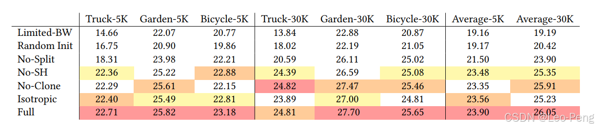
论文给出如下几个结论：

1. 从SFM进行初始化非常重要；
2. 训练过程中对3D Gaussian进行Clone和Split确实可以使得训练效果更好；
3. Unlimited Depth Complexity of Splats with Gradients（我理解指的是通过上述代码中last_contributor自适应地控制梯度回传到哪些3D Gaussian中）可以加速收敛过程；
4. 各向异性的协方差可以提升渲染效果；
5. 球谐函数具备视角连续性，使用球谐函数对渲染效果同样提升；