
阅读量:0
Step 1: Loading the data
import numpy as np import pandas as pd import matplotlib.pyplot as plt import torch.nn as nn import torch from torch.autograd import Variable from torch.utils.data import Dataset, DataLoader # Importing the training set dataset = pd.read_csv('HistoricalData_1719412320530.csv') dataset.head(10)
dataset.info() <class 'pandas.core.frame.DataFrame'> RangeIndex: 2516 entries, 0 to 2515 Data columns (total 6 columns): # Column Non-Null Count Dtype --- ------ -------------- ----- 0 Date 2516 non-null object 1 Close/Last 2516 non-null object 2 Volume 2516 non-null int64 3 Open 2516 non-null object 4 High 2516 non-null object 5 Low 2516 non-null object dtypes: int64(1), object(5) memory usage: 118.1+ KB # change time order dataset['Date'] = pd.to_datetime(dataset['Date'], format='%m/%d/%Y') # Sort the DataFrame in ascending order dataset = dataset.sort_values(by='Date', ascending=True) # Reset index if necessary dataset = dataset.reset_index(drop=True) dataset.head(5)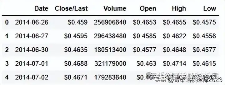
dataset['Close/Last'] = dataset['Close/Last'].str.replace('$', '').astype(float) dataset.head(5)
dataset_cl = dataset['Close/Last'].values # Feature Scaling from sklearn.preprocessing import MinMaxScaler sc = MinMaxScaler(feature_range = (0, 1)) # scale the data dataset_cl = dataset_cl.reshape(dataset_cl.shape[0], 1) dataset_cl = sc.fit_transform(dataset_cl) dataset_cl array([[2.91505500e-04], [2.95204809e-04], [3.24799276e-04], ..., [9.33338463e-01], [8.70746165e-01], [9.29787127e-01]])Step 2: Cutting time series into sequences (Sliding Window)
input_size = 7 # Create a function to process the data into 7 day look back slices # lb is window size def processData(data, lb): X, y = [], [] # X is input vector, Y is output vector for i in range(len(data) - lb - 1): X.append(data[i: (i + lb), 0]) y.append(data[(i + lb), 0]) return np.array(X), np.array(y) X, y = processData(dataset_cl, input_size)Step 3: Split training and testing sets
X_train, X_test = X[:int(X.shape[0]*0.80)], X[int(X.shape[0]*0.80):] y_train, y_test = y[:int(y.shape[0]*0.80)], y[int(y.shape[0]*0.80):] print(X_train.shape[0]) print(X_test.shape[0]) print(y_train.shape[0]) print(y_test.shape[0]) # reshaping X_train = np.reshape(X_train, (X_train.shape[0], 1, X_train.shape[1])) X_test = np.reshape(X_test, (X_test.shape[0], 1, X_test.shape[1])) 2006 502 2006 502Step 4: Build and run an RNN regression model
class RNN(nn.Module): def __init__(self, i_size, h_size, n_layers, o_size, dropout=0.1, bidirectional=False): super().__init__() # super(RNN, self).__init__() self.num_directions = bidirectional + 1 # LSTM module self.rnn = nn.LSTM( input_size = i_size, hidden_size = h_size, num_layers = n_layers, dropout = dropout, bidirectional = bidirectional ) # self.relu = nn.ReLU() # Output layer self.out = nn.Linear(h_size, o_size) def forward(self, x, h_state): # r_out contains the LSTM output at each time step, and hidden_state # contains the hidden and cell states after processing the entire sequence. r_out, hidden_state = self.rnn(x, h_state) hidden_size = hidden_state[-1].size(-1) # Convert dimension of r_out (-1 denotes it depends on other parameters) r_out = r_out.view(-1, self.num_directions, hidden_size) # r_out = self.relu(r_out) outs = self.out(r_out) return outs, hidden_state # Global setting INPUT_SIZE = input_size # LSTM input size HIDDEN_SIZE = 256 NUM_LAYERS = 3 # LSTM 'stack' layer OUTPUT_SIZE = 1 # Hyper parameters learning_rate = 0.001 num_epochs = 300 rnn = RNN(INPUT_SIZE, HIDDEN_SIZE, NUM_LAYERS, OUTPUT_SIZE, bidirectional=False) rnn.cuda() optimiser = torch.optim.Adam(rnn.parameters(), lr=learning_rate) criterion = nn.MSELoss() hidden_state = None rnn RNN( (rnn): LSTM(7, 256, num_layers=3, dropout=0.1) (out): Linear(in_features=256, out_features=1, bias=True) ) history = [] # save loss in each epoch # .cuda() copies element to the GPU memory X_test_cuda = torch.tensor(X_test).float().cuda() y_test_cuda = torch.tensor(y_test).float().cuda() # Use all the data in one batch inputs_cuda = torch.tensor(X_train).float().cuda() labels_cuda = torch.tensor(y_train).float().cuda() # training for epoch in range(num_epochs): # Train mode rnn.train() output, _ = rnn(inputs_cuda, hidden_state) # print(output.size()) loss = criterion(output[:,0,:].view(-1), labels_cuda) optimiser.zero_grad() loss.backward() # back propagation optimiser.step() # update the parameters if epoch % 20 == 0: # Convert train mode to evaluation mode (disable dropout) rnn.eval() test_output, _ = rnn(X_test_cuda, hidden_state) test_loss = criterion(test_output.view(-1), y_test_cuda) print('epoch {}, loss {}, eval loss {}'.format(epoch, loss.item(), test_loss.item())) else: print('epoch {}, loss {}'.format(epoch, loss.item())) history.append(loss.item()) # iterate over all the learnable parameters in the model, which include the # weights and biases of all layers in the model # (both the LSTM layers and the final linear layer) for param in rnn.parameters(): print(param.data)Step 5: Checking model performance
plt.plot(history) # dplt.plot(history.history['val_loss'])
# X_train_X_test = np.concatenate((X_train, X_test),axis=0) # hidden_state = None rnn.eval() # test_inputs = torch.tensor(X_test).float().cuda() test_predict, _ = rnn(X_test_cuda, hidden_state) test_predict_cpu = test_predict.cpu().detach().numpy() plt.plot(sc.inverse_transform(y_test.reshape(-1,1))) plt.plot(sc.inverse_transform(test_predict_cpu.reshape(-1,1))) plt.legend(['y_test','test_predict_cpu'], loc='center left', bbox_to_anchor=(1, 0.5))
# plot original data plt.plot(sc.inverse_transform(y.reshape(-1,1)), color='k') # train_inputs = torch.tensor(X_train).float().cuda() train_pred, hidden_state = rnn(inputs_cuda, None) train_pred_cpu = train_pred.cpu().detach().numpy() # use hidden state from previous training data test_predict, _ = rnn(X_test_cuda, hidden_state) test_predict_cpu = test_predict.cpu().detach().numpy() # plt.plot(scl.inverse_transform(y_test.reshape(-1,1))) split_pt = int(X.shape[0] * 0.80) + 7 # window_size plt.plot(np.arange(7, split_pt, 1), sc.inverse_transform(train_pred_cpu.reshape(-1,1)), color='b') plt.plot(np.arange(split_pt, split_pt + len(test_predict_cpu), 1), sc.inverse_transform(test_predict_cpu.reshape(-1,1)), color='r') # pretty up graph plt.xlabel('day') plt.ylabel('price of Nvidia stock') plt.legend(['original series','training fit','testing fit'], loc='center left', bbox_to_anchor=(1, 0.5)) plt.show()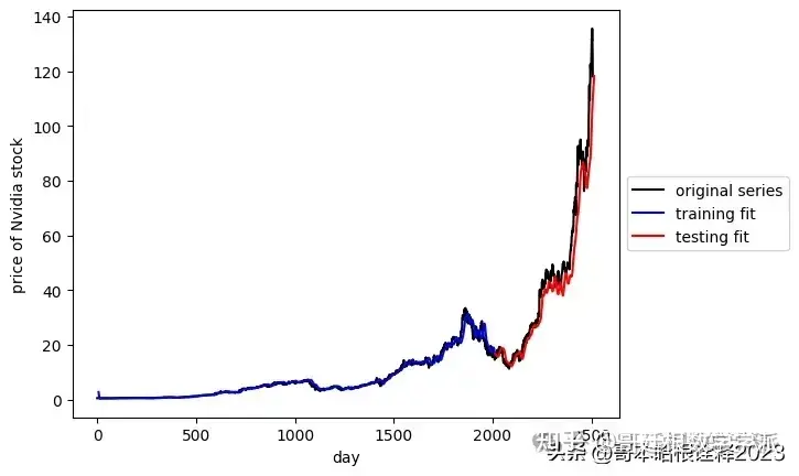
MMSE = np.sum((test_predict_cpu.reshape(1,X_test.shape[0])-y[2006:])**2)/X_test.shape[0] print(MMSE) 0.0018420128176938062 担任《Mechanical System and Signal Processing》审稿专家,担任《中国电机工程学报》,《控制与决策》等EI期刊审稿专家,擅长领域:现代信号处理,机器学习,深度学习,数字孪生,时间序列分析,设备缺陷检测、设备异常检测、设备智能故障诊断与健康管理PHM等。 知乎学术咨询:https://www.zhihu.com/consult/people/792359672131756032?isMe=1