
阅读量:0
原文链接:模式植物构建orgDb数据库 | 以org.Slycompersicum.eg.db为例

本期教程
一步构建模式植物OrgDb数据库
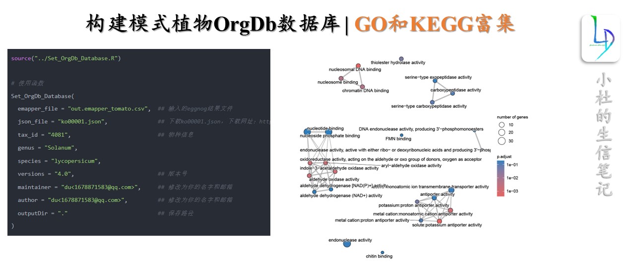
source("../Set_OrgDb_Database.R") # 使用函数 Set_OrgDb_Database( emapper_file = "out.emapper_tomato.csv", ## 输入的eggnog结果文件 json_file = "ko00001.json", ## 下载ko00001.json,下载网址:https://www.genome.jp/kegg-bin/get_htext?ko00001 tax_id = "4081", ## 物种信息 genus = "Solanum", species = "lycopersicum", versions = "4.0", ## 版本号 maintainer = "du<1678871583@qq.com>", ## 修改为你的名字和邮箱 author = "du<1678871583@qq.com>", ## 修改为你的名字和邮箱 outputDir = "." ## 保存路径 ) 获得本期教程文本文档,在后台回复:20240802。注意:一步构建模式植物OrgDb数据库Set_OrgDb_Database()函数教程可在社群中获得。请大家看清楚回复关键词,每天都有很多人回复错误关键词,我这边没时间和精力一一回复。
写在前面
前期,我们发表过模式植物GO背景基因集制作,这些教程也算是比较“经济实惠”、且常用的。在我们制作分析是会遇到的问题,随着前面教程推出,也有同学咨询如何制作KEGG背景文件。今天,自己也查了相关的教程,进行整理一下。最开始的目标是,将我们注释文件进行本地打包建库,使用时就会更加的方便。但是,在此过程中,出现一些问题,目前还未解决。那就安排到下一期的内容吧。
一、使用ggNOG-mapper仅需注释
1 模式植物KEGG注释
本次使用Egg-mapper进行注释,网页版可以支持proteins/CDS/genomic/Metagenomic和seeds文件格式。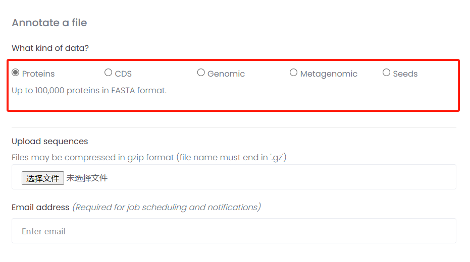
1.1 下载模式植物序列
本次事例中,我们使用Proteins文件进行注释。使用番茄(tomato)蛋白序列,你可以使用其它序列。
wget https://solgenomics.net/ftp/genomes/Solanum_lycopersicum/annotation/ITAG4.0_release/ITAG4.0_proteins.fasta 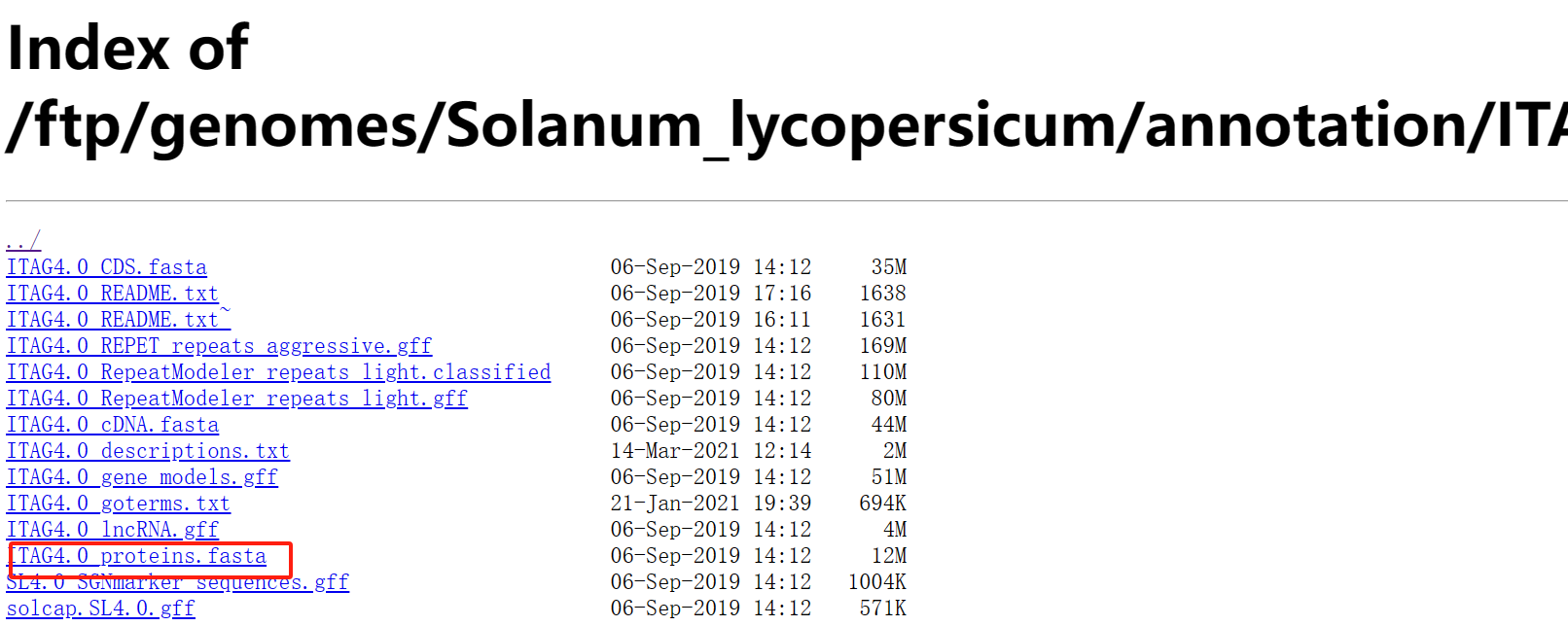
1.2 上传到ggNOG-mapper
egg-mapper网址
http://eggnog-mapper.embl.de/ 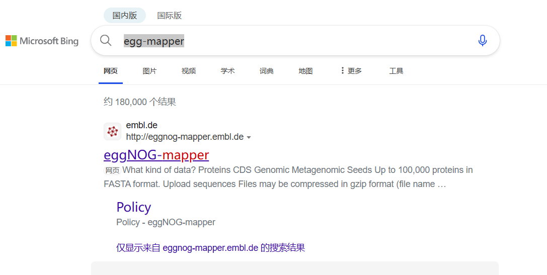
上传蛋白序列
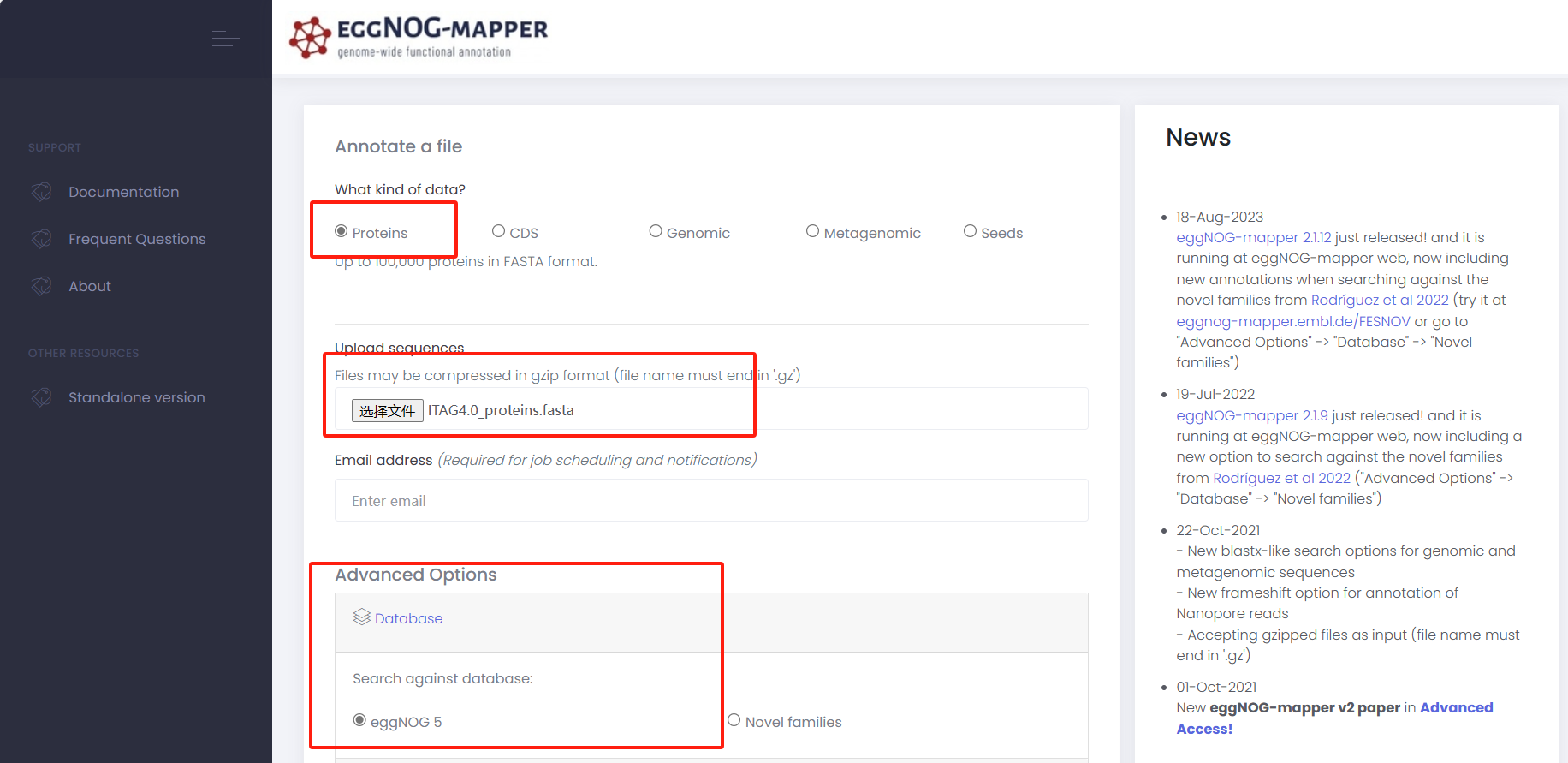
输入邮箱
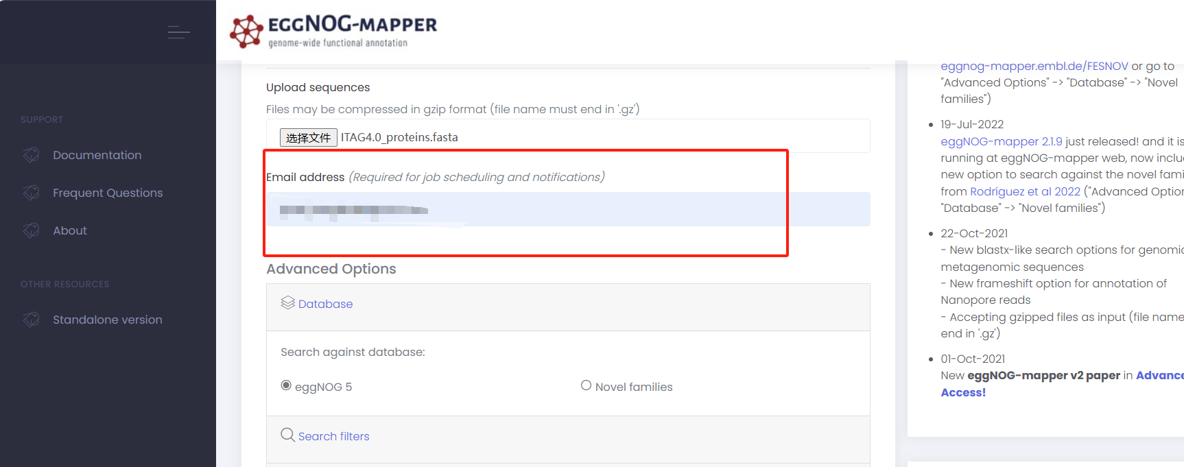
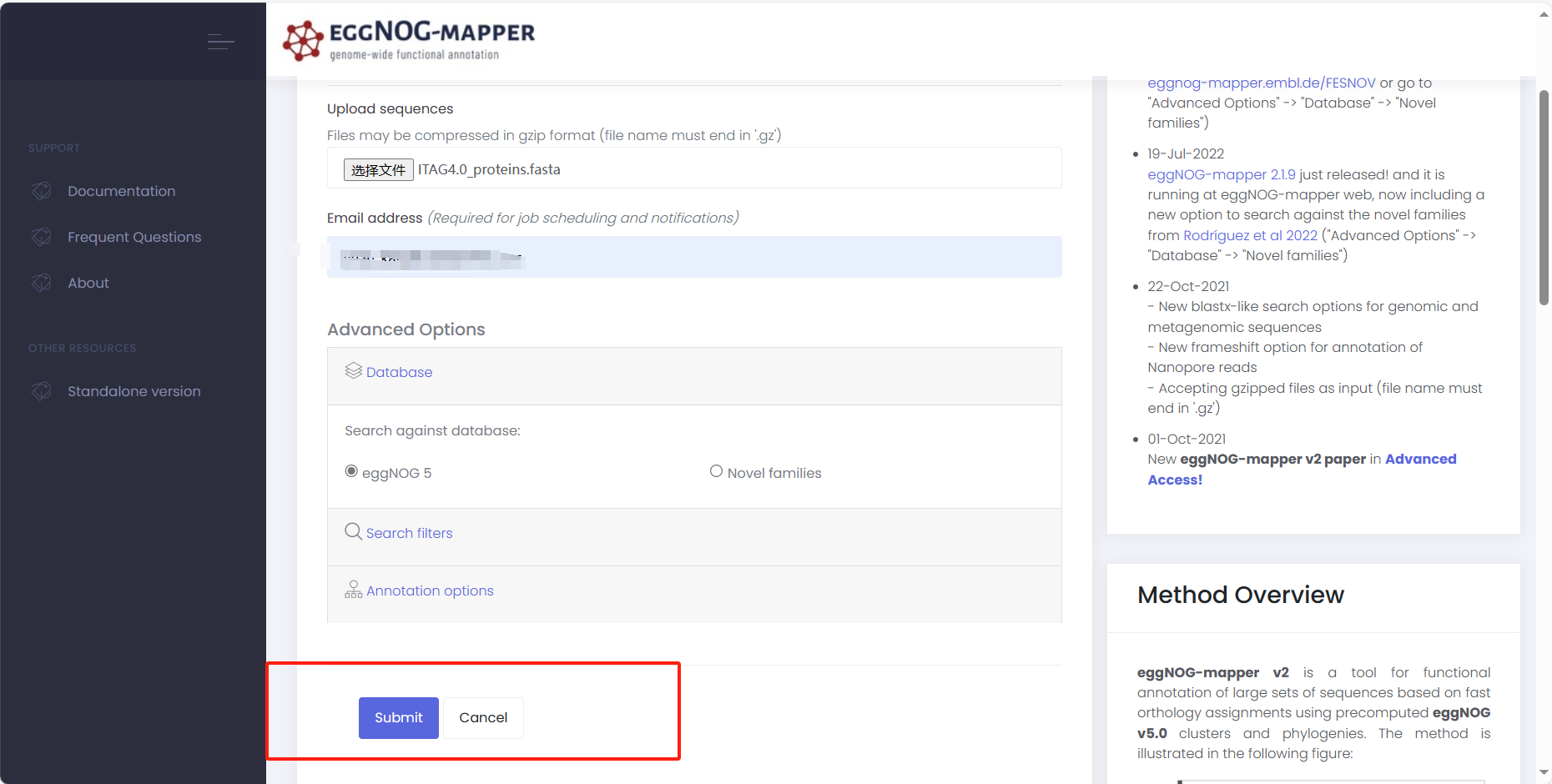
提交
邮箱中收到eggNOG-mapper发送的邮件
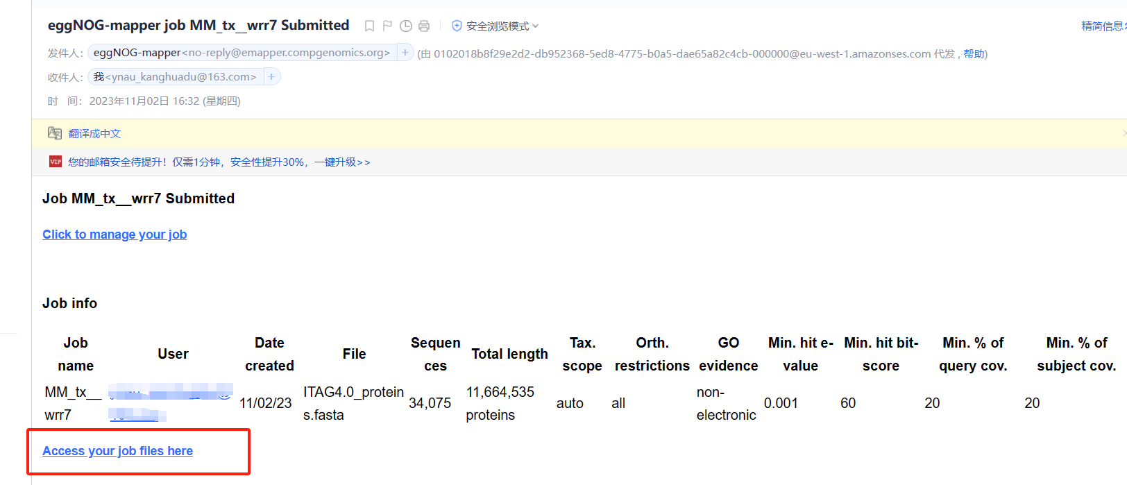
开始运行【重点】
在我们收到邮件时,很多同学可能会认为此任务已经开始(PS:自己也是这么认为的)。但是,我们需要点击Click to manage your job进去工作台,点击start job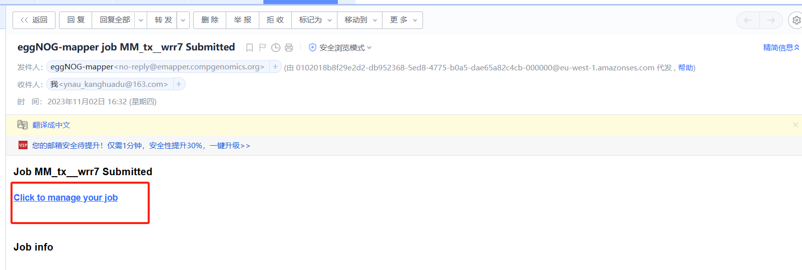
进入工作台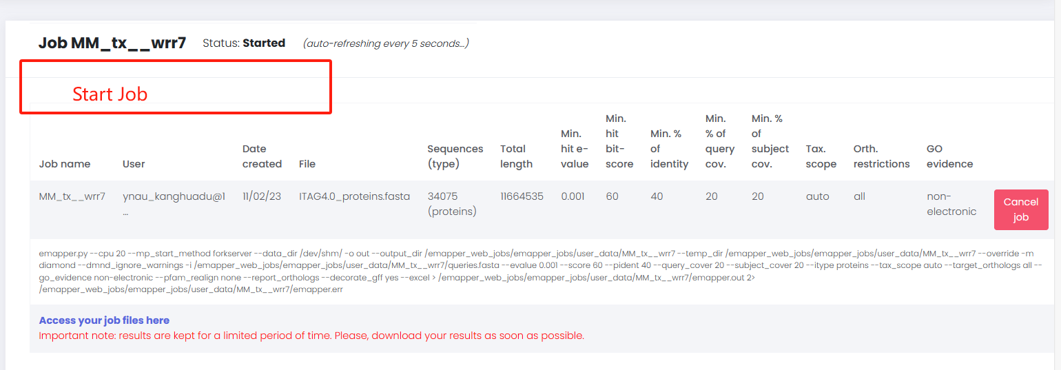
开始运行工作文件后台界面
1.3 下载注释文件
若你提交的任务结束,可以到工作任务后台下载数据。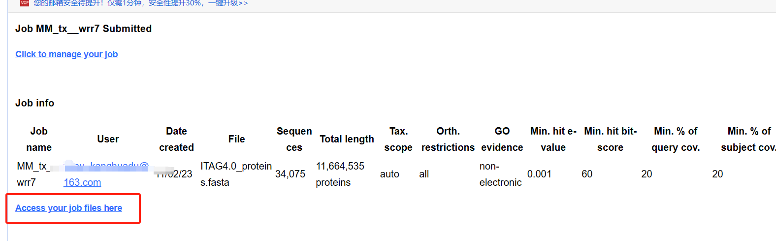
下载数据
2 本地运行
2.1安装egg-mapper软件
- conda或mamba安装
mamba install -c bioconda -c conda-forge eggnog-mapper or conda install -c bioconda -c conda-forge eggnog-mapper 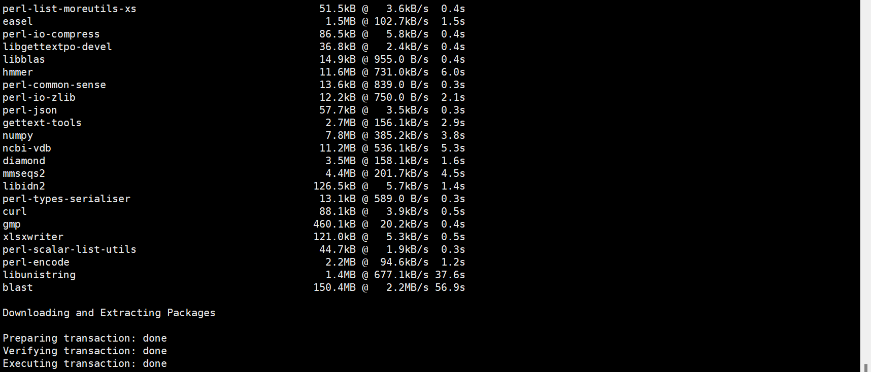
- 源码安装
下载网址: https://github.com/eggnogdb/eggnog-mapper/releases/tag/2.1.12 
3. 帮助文档网址
https://github.com/eggnogdb/eggnog-mapper/wiki/ ## v2.1.5版本帮助文档 https://github.com/eggnogdb/eggnog-mapper/wiki/eggNOG-mapper-v2.1.5-to-v2.1.12#user-content-Software_Requirements 2.2 安装软件需求
- Python 3.7 (or greater) - BioPython 1.76 (python package) (BioPython 1.78 should work since emapper version 2.1.7) - psutil 5.7.0 (python package) - xlsxwriter 1.4.3 (python package), only if using the --excel option - wget (linux command, required for downloading the eggNOG-mapper databases with download_eggnog_data.py, and to create new Diamond/MMseqs2 databases with create_dbs.py) - sqlite (>=3.8.2) 2.3 硬盘储存需求
- eggNOG annotation databases:~40 GB
- eggNOG sequences:~9 GB
- MMseqs2 database of eggNOG sequences:~11 GB(~86 GB if MMseqs2 index is created)
- PFAM database:~3 GB
2.4 内存需求
- Using --dbmem loads the whole eggnog.db sqlite3 annotation database during the annotation step, and therefore requires ~44 GB of memory. - Using the --num_servers option when running HMMER in server mode (a.k.a. hmmgpmd, which is used for -m hmmer --usemem, --pfam_realign denovo or hmm_server.py) loads the HMM database as many times as specified in the argument (e.g. --pfam_realign denovo --num_servers 2 loads the PFAM database into memory twice, with up to roughly 2 GB per instance). 2.5 数据库下载
下载网址:http://eggnog6.embl.de/#/app/downloads
在eggnog_6.0版本中提供此下载数据信息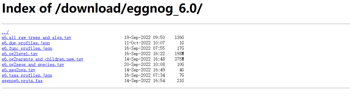
使用软件自带的脚本下载数据库:
download_eggnog_data.py -h 注意,我们这里使用conda或mamba,以及添加到$PATH路径中,可以直接运行。若你使用源码安装,及未添加路径,需求添加python /PATH/download_eggnog_data.py -h运行。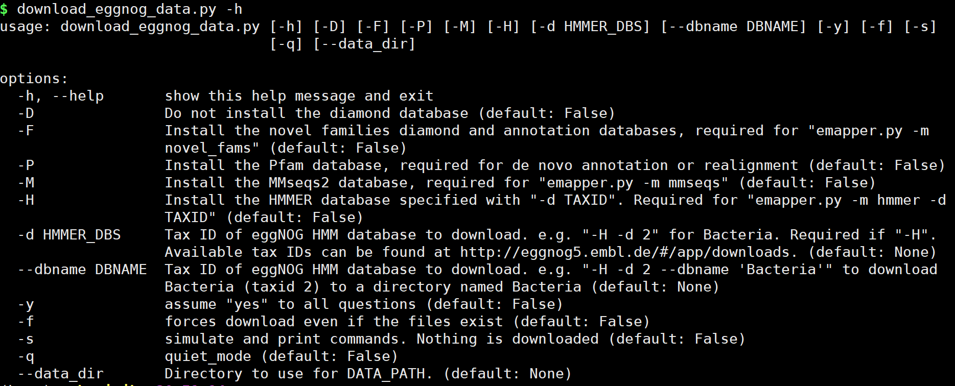
下载数据库整体命令:
download_eggnog_data.py --data_dir /home/Data/DataBase/Eggno_Database/ -y -F -D -H 参数选择:
options: -h, --help show this help message and exit -D Do not install the diamond database (default: False) -F Install the novel families diamond and annotation databases, required for "emapper.py -m novel_fams" (default: False) -P Install the Pfam database, required for de novo annotation or realignment (default: False) -M Install the MMseqs2 database, required for "emapper.py -m mmseqs" (default: False) -H Install the HMMER database specified with "-d TAXID". Required for "emapper.py -m hmmer -d TAXID" (default: False) -d HMMER_DBS Tax ID of eggNOG HMM database to download. e.g. "-H -d 2" for Bacteria. Required if "-H". Available tax IDs can be found at http://eggnog5.embl.de/#/app/downloads. (default: None) --dbname DBNAME Tax ID of eggNOG HMM database to download. e.g. "-H -d 2 --dbname 'Bacteria'" to download Bacteria (taxid 2) to a directory named Bacteria (default: None) -y assume "yes" to all questions (default: False) -f forces download even if the files exist (default: False) -s simulate and print commands. Nothing is downloaded (default: False) -q quiet_mode (default: False) --data_dir Directory to use for DATA_PATH. (default: None) 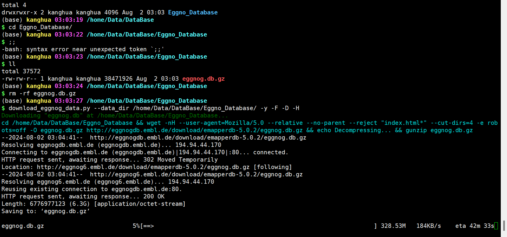
2.6 运行
HMMER方法
本地检索细菌数据库
-i输入、—output输出文件前缀、-d指定数据库数据、—data_dir指定数据库位置
python emapper.py -i test/polb.fa --output polb_bact -d bact --data_dir ~/data/db/eggnog diamond方法-m指定diamond方法,默认为hmmer方法。diamond在多于千条序列时才会体现速度优势,少量序列会感觉非常慢,而且结果也没有hmmer的更准确,尤其是对远源注释方面。
python emapper.py -i test/polb.fa --output diamond_bact_ -d bact --data_dir ~/data/db/eggnog -m diamond 此外,作者也在推文或帮助文档中说明,可以增加内存和线程数量,使用--usemem增加内存,使用--cup增加线程数,--override是强制覆盖结果。
python emapper.py -i test/polb.fa --output diamond_bact_ -d bact --data_dir ~/data/db/eggnog --usemem --cpu 10 --override -m diamond 跟多细节请查看官网即可:
https://github.com/eggnogdb/eggnog-mapper/wiki/eggNOG-mapper-v2.1.5-to-v2.1.12#user-content-Software_Requirements 对于使用在线eggNOG-mapper还是自己在服务器中进行搭建呢?
对于这个问题,每个人分析的环境不同以及资源不同,我们根据自己的环境和资源进行合理调整即可。
- 若手中的有充足资源服务器,可以自己搭建,有利于后续流程的搭建和分析。
- 若自己手中并未有那么充足资源,其实使用在线的分析也可以,足够使用。
3 结果分析
运行成功后,我们获得一下注释文件信息。如何操作,就成为后续分析重点。类似思路,可以依据模式植物GO背景基因集制作。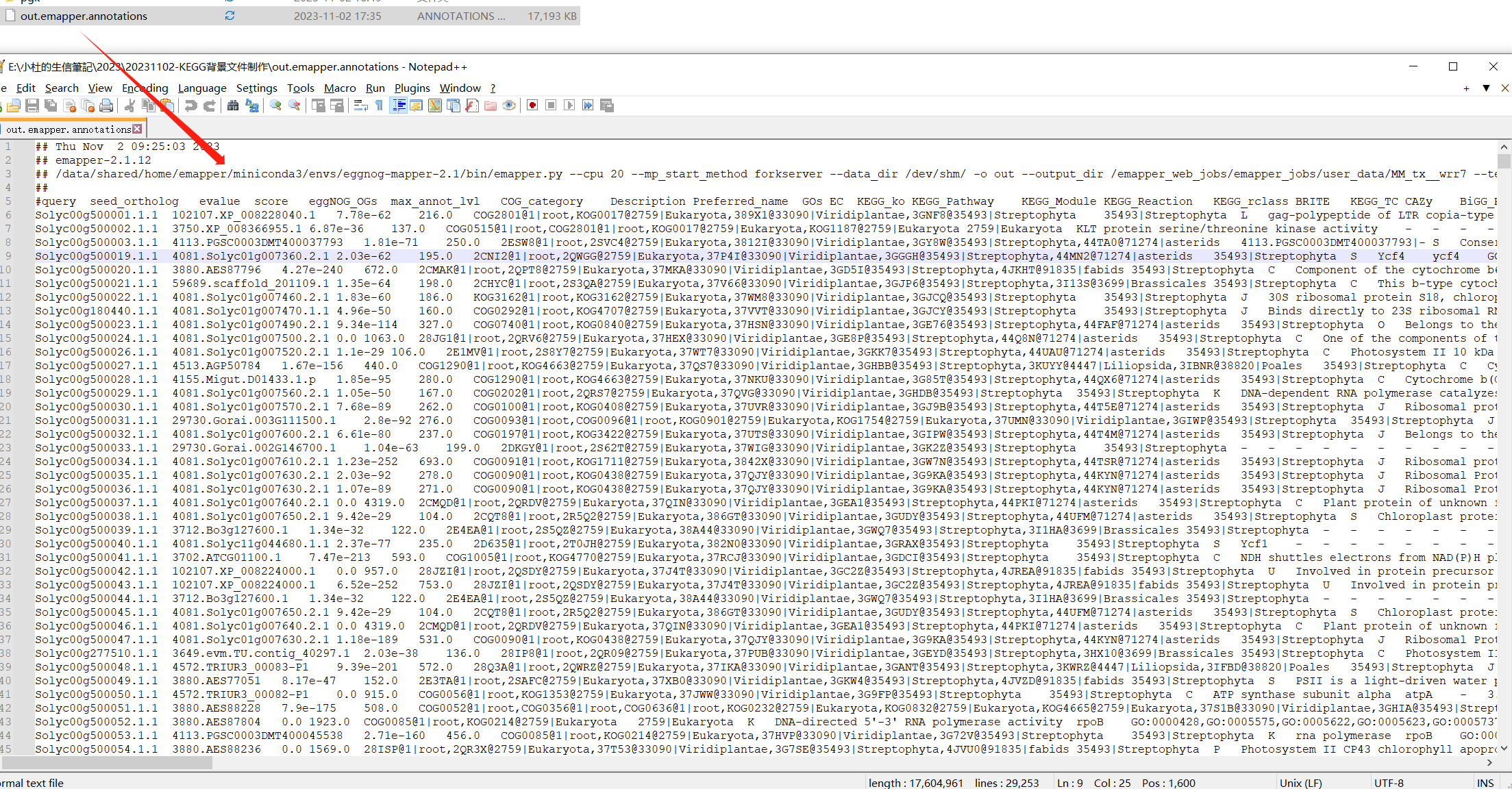
标注的信息就是我们制作KEGG背景文件重要的信息。
我们在这里可以发现,在egg-mapper中注视到GO ID,那么是不是GO背景文件也可以使用这个文件进行制作呢??与前期的教程有何差异呢??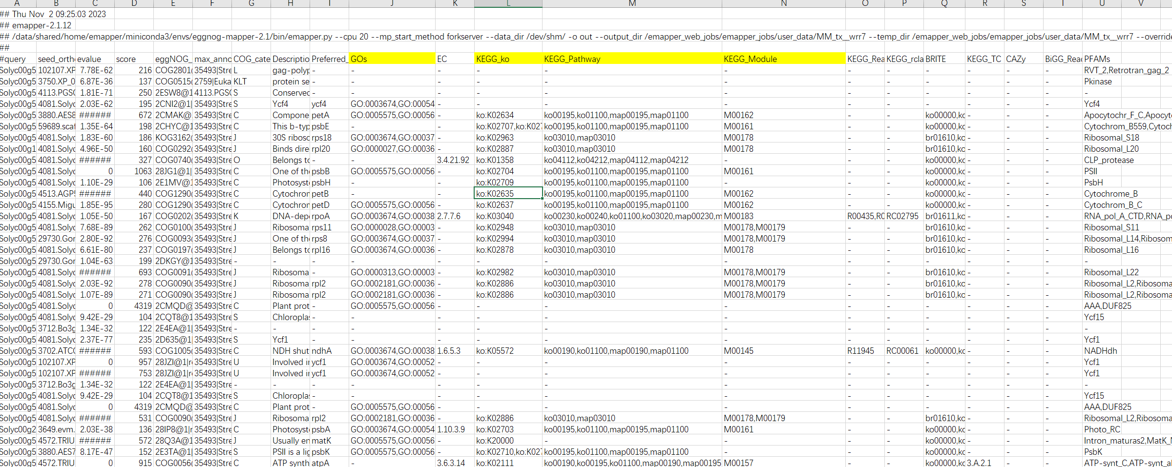
结果解读:
第一列:查询序列名称 第二列:eggNOG种子序列 第三列:eggNOG种子序列 evalue 第四列:eggNOG种子序列 bit score 第五列:匹配的OGs 第六列:最大的OG分类等级 第七列:COG功能分类 第八列:OGs最低分类等级物种描述 第九列:首选名称 第十列:GOs, 预测的GO,逗号分隔 第十一列:EC,预测额EC 第十二列:KEGG_KO: 预测的KO 第十三列:KEGG_Pathway:预测的ko通路 第十四列:KEGG_Module:预测的ko功能单元 第十五列:KEGG_Reaction:预测的酶促反应 第十六列:KEGG_rclass:预测的ko相关类 第十七列:BRITE:预测的brite功能分类 第十八列:KEGG_TC 第十九列:CAZy:预测的碳水化合物活性酶 第二十列:BiGG_Reaction:BiGG代谢反应预测 第二十一列:PFAMs:pfam蛋白预测 我们了解整个注释文件的信息,如何来提取对应的数据集分析呢?
3.1 使用TBtols进行富集
- 打开
Tbtools中的eggNOG-mapper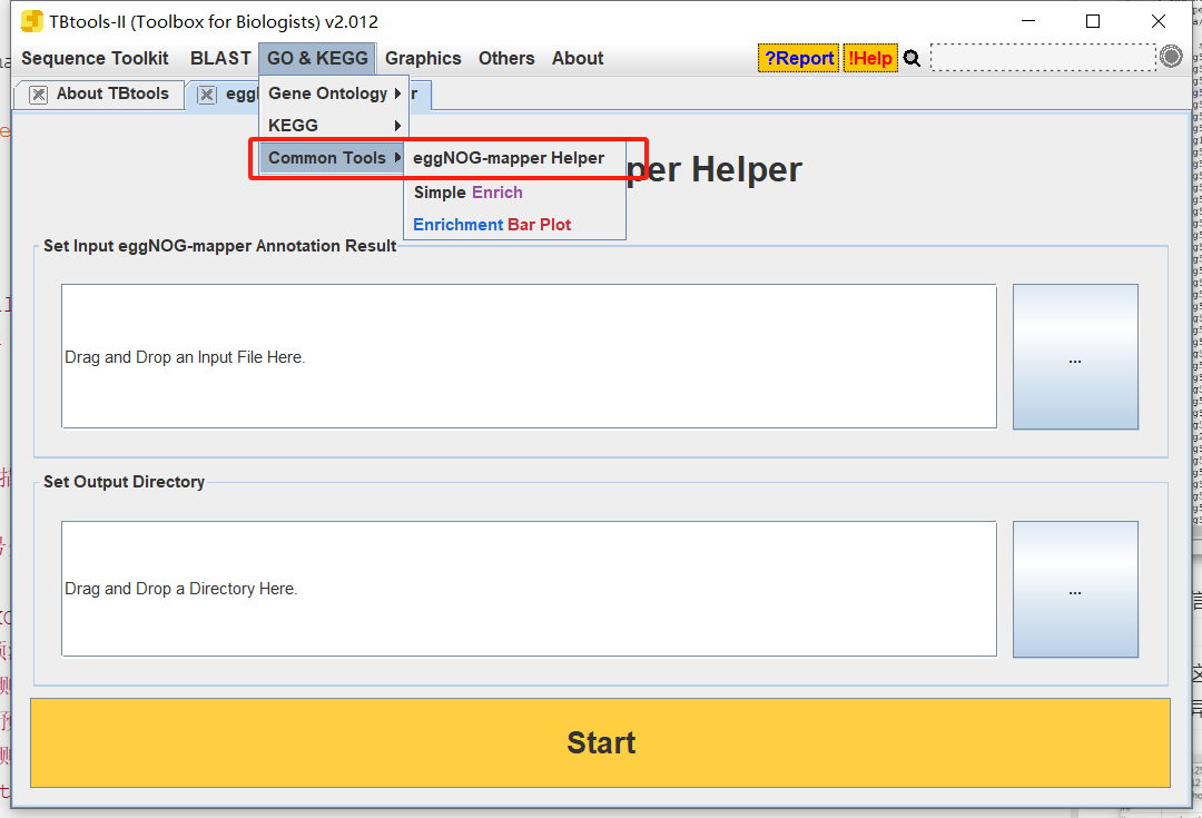
- 将注释文件拖拽进去
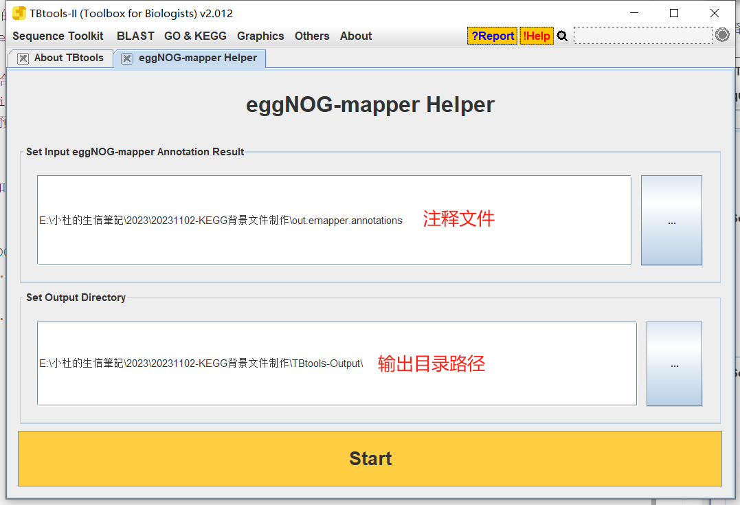
- 输出结果
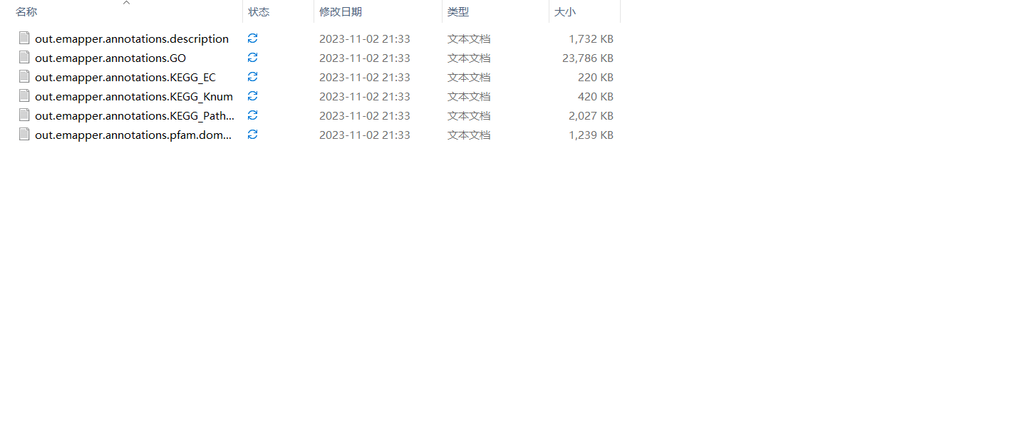
输出文件,将注释ID与每个的GO ID或KEGG ID进行整理,直接生成一个背景文件信息,可以直接上传到云平台中进行分析。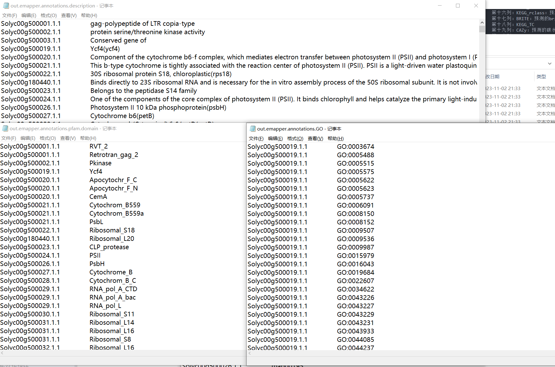
3.使用TBtools进行富集
TBtools为什么受这么多人的欢迎,功能很强大。基本把你遇到的问题,都会提供解决。
(1)下载.KEGG.BackEnd文件和go-basic.obo
下载网址:
https://tbtools.cowtransfer.com/s/566e88227a0045 (2)运行
依次输入进行做好的注释文件和的差异基因即可进行富集
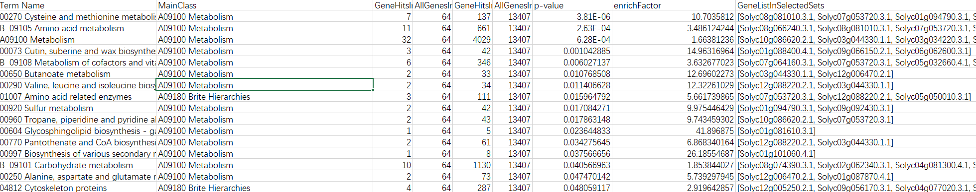
(3)结果
输出两个结果,一个是全部结果,另一个是过滤后的结果。

(4)绘制结果图形
绘制图形,可以根据自己的需求进绘制即可。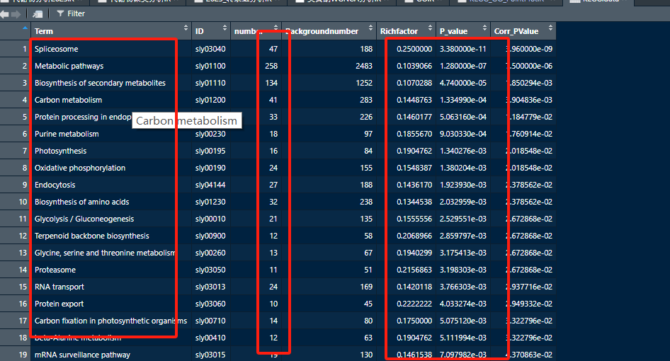
根据自己需求进行整理即可。
KEGG.data <- read.csv("KEGG_Enrichment_plotdata.csv", header = T) names(KEGG.data) <- c("Term","ID","number", "Backgroundnumber","Richfactor","P_value", "Corr_PValue") head(KEGG.data) ggplot(KEGG.data, aes(x = number, y = Term))+ geom_bar(stat = "identity", position = "dodge", color = "black")+ xlab("Gene number")+ ylab("")+ theme_classic()+theme(legend.title = element_blank()) 
ggplot(KEGG.data, aes(x = Richfactor, y = Term))+ geom_point(aes(size = number, color = -1*log10(Corr_PValue)))+ scale_color_gradient(low = "#0000ff", high = "#ff0033")+ labs(color = expression(-log[10](PValue)), size = "Gene number", x = "Rich Factor", y = "", title = "KEGG Pathway Enrichment")+ theme(legend.background = element_blank())+theme_bw()+ ## theme_bw() 去掉背景 theme(axis.text = element_text(face = "bold",color = "black", size = 7)+ ## 修改字体大小,根据自己实际情况修改 theme( axis.text = element_text(size = 12, family = "Arial", color = "black"), axis.title = element_text(size = 14, family = "Arial", color = "black"), legend.text = element_text(size = 12, family = "Arial", color = "black"), legend.title = element_text(size = 14, family = "Arial", color = "black")) ) 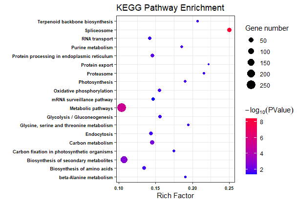
参考:
- https://mp.weixin.qq.com/s/Ii-pB0JEDt_pRRKPyq3RLw
- https://mp.weixin.qq.com/s/kIf6C2u3FID3ZeLtsB4eZQ
二、构建OrgDb数据库
我们上面的操作是将构建出来背景文件文件使用云平台或TBtools工具进行功能富集,那么若是使用clusterProfiler等包进行本地富集,就需要构建OrgDb数据库。
我们这里基于网上的教程资源,整理如何制作模式植物本地OrgDB数据库。在文末会标注的相关参考资源,在此也感谢各位知识分享博主的分享。
2.1 整理ggNOG-mapper注释文件
在注释文件中,会有很多列信息,我们可以做直接导入数据(PS:可能导入时会报错)。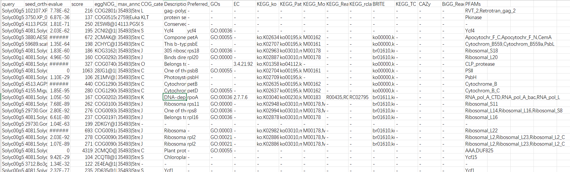
emapper <- read.table("out.emapper_tomato.txt", header = T, sep = "\t") 若是报错,我们可以在本地提取相关的信息即可。我们所需的信息就只有ID,GO,KEGG信息列。
emapper <- read.csv("out.emapper_tomato.csv",header = T, check.names = F) 2.2 温馨提示
本教程,我们会提供分布式的步骤教程,大家可以直接跟随教程直接做即可。每个步骤,我们都会有详细的说明。此外,我们也会提供一步式教程,方便我们后期的制作 ,一步式教程,在我们的社群中可以查看。
模式植物本地OrgDb数据库制作
- 导入相关的R包
library(clusterProfiler) library(tidyverse) library(stringr) library(KEGGREST) library(AnnotationForge) library(clusterProfiler) library(dplyr) library(jsonlite) library(purrr) library(RCurl) options(stringsAsFactors = F) - 导入数据
setwd("D:\\小杜的生信笔记\\2024\\20240802_模式植物构建OegDB数据库") emapper <- read.csv("out.emapper_tomato.csv",header = T, check.names = F) head(emapper) 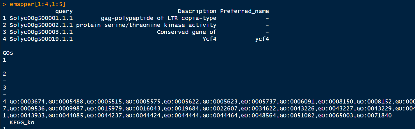
将缺省值替换为NA
emapper[emapper==""]<-NA - 提取GO信息
gene_info <- emapper %>% dplyr::select(GID = query,GENENAME = Preferred_name) %>% na.omit() gos <- emapper %>% dplyr::select(query, GOs) %>% na.omit() head(gos) - 构建空的gene2go数据框
gene2go = data.frame(GID =character(), GO = character(), EVIDENCE = character()) 排顺整理,需要花费一定时间。
for (row in 1:nrow(gos)) { the_gid <- gos[row, "query"][[1]] the_gos <- str_split(gos[row,"GOs"], ",", simplify = FALSE)[[1]] df_temp <- data_frame(GID=rep(the_gid, length(the_gos)), GO = the_gos, EVIDENCE = rep("IEA", length(the_gos))) gene2go <- rbind(gene2go, df_temp) } 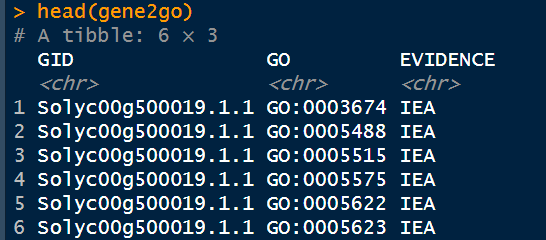
5. 删除NA行
gene2go$GO[gene2go$GO=="-"]<-NA gene2go<-na.omit(gene2go) - 提取KEGG信息
在这里,我们提取的是KO号列。
#把Emapper中的query列、KEGG_ko列提出出来 gene2ko <- emapper %>% dplyr::select(GID = query, Ko = KEGG_ko) %>% na.omit() #将gene2ko的Ko列中的“Ko:”删除,不然后面找pathway会报错 gene2ko$Ko <- gsub("ko:","",gene2ko$Ko) head(gene2ko) > head(gene2ko) GID Ko 1 Solyc00g500001.1.1 - 2 Solyc00g500002.1.1 - 3 Solyc00g500003.1.1 - 4 Solyc00g500019.1.1 - 5 Solyc00g500020.1.1 K02634 6 Solyc00g500021.1.1 K02707,K02713 - 下载KO的json文件,下载地址https://www.genome.jp/kegg-bin/get_htext?ko00001
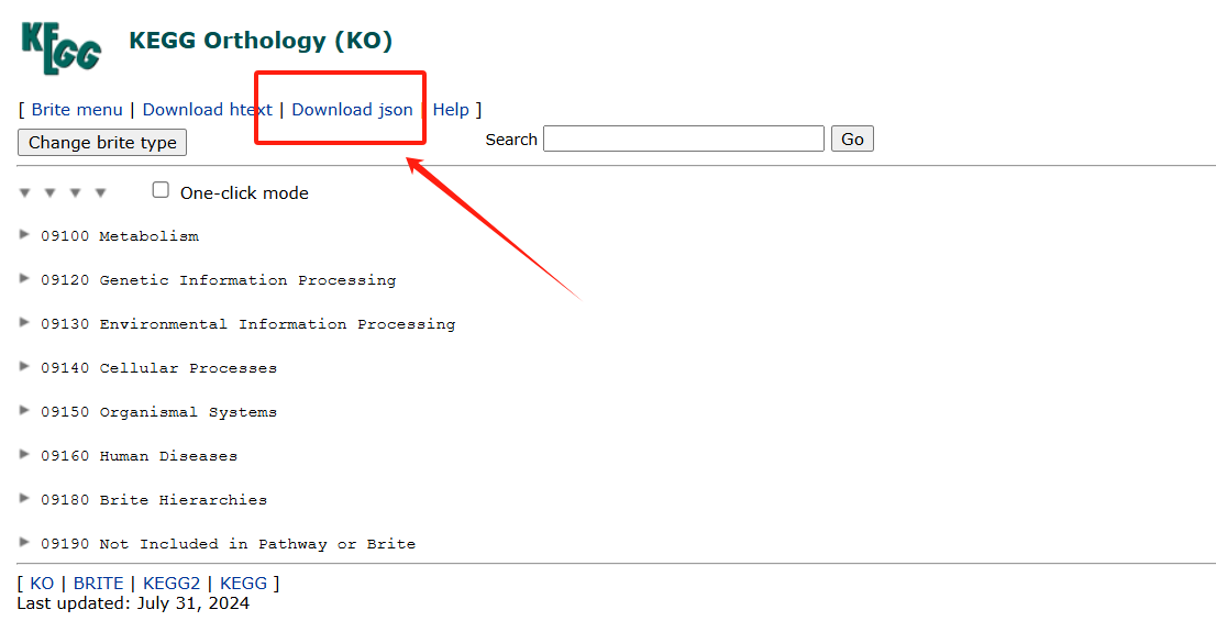
下载后,放在路劲文件夹中。
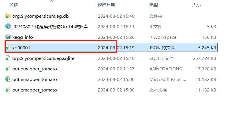
- 运行一下代码,本地创建
kegg_info.RData文件
update_kegg <- function(json = "ko00001.json") { pathway2name <- tibble(Pathway = character(), Name = character()) ko2pathway <- tibble(Ko = character(), Pathway = character()) kegg <- fromJSON(json) for (a in seq_along(kegg[["children"]][["children"]])) { A <- kegg[["children"]][["name"]][[a]] for (b in seq_along(kegg[["children"]][["children"]][[a]][["children"]])) { B <- kegg[["children"]][["children"]][[a]][["name"]][[b]] for (c in seq_along(kegg[["children"]][["children"]][[a]][["children"]][[b]][["children"]])) { pathway_info <- kegg[["children"]][["children"]][[a]][["children"]][[b]][["name"]][[c]] pathway_id <- str_match(pathway_info, "ko[0-9]{5}")[1] pathway_name <- str_replace(pathway_info, " \\[PATH:ko[0-9]{5}\\]", "") %>% str_replace("[0-9]{5} ", "") pathway2name <- rbind(pathway2name, tibble(Pathway = pathway_id, Name = pathway_name)) kos_info <- kegg[["children"]][["children"]][[a]][["children"]][[b]][["children"]][[c]][["name"]] kos <- str_match(kos_info, "K[0-9]*")[,1] ko2pathway <- rbind(ko2pathway, tibble(Ko = kos, Pathway = rep(pathway_id, length(kos)))) } } } save(pathway2name, ko2pathway, file = "kegg_info.RData") } ##'@本地创建kegg_info.RData文件 update_kegg() ##'@载kegg_info.RData load(file = "kegg_info.RData") - 根据gene2ko中的ko信息将ko2pathway中的pathway列提取出来
gene2pathway <- gene2ko %>% left_join(ko2pathway,by = "Ko") %>% dplyr::select(GID, Pathway) %>% na.omit() 注意:在此步骤,可能会出现警告提示,大家忽略即可,不要以为是报错信息。

- 在网站https://www.ncbi.nlm.nih.gov/taxonomy上查询物种信息
** 进入网站:**
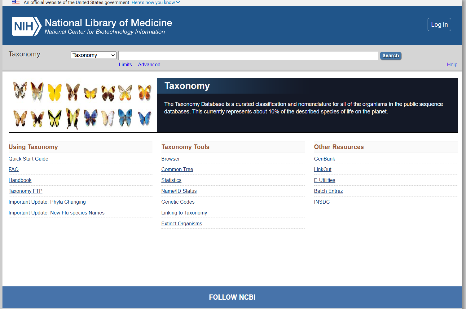
搜索物种
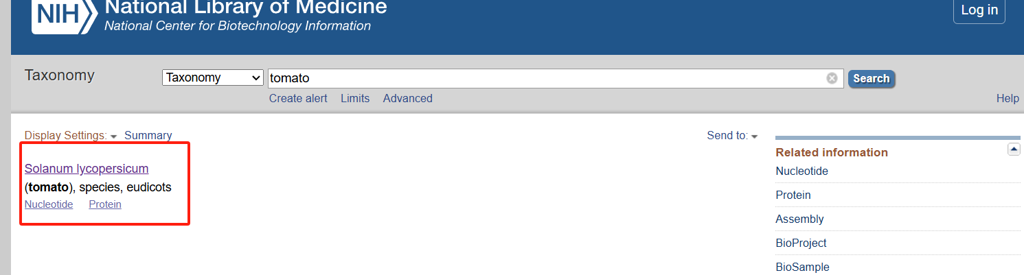
点进进去
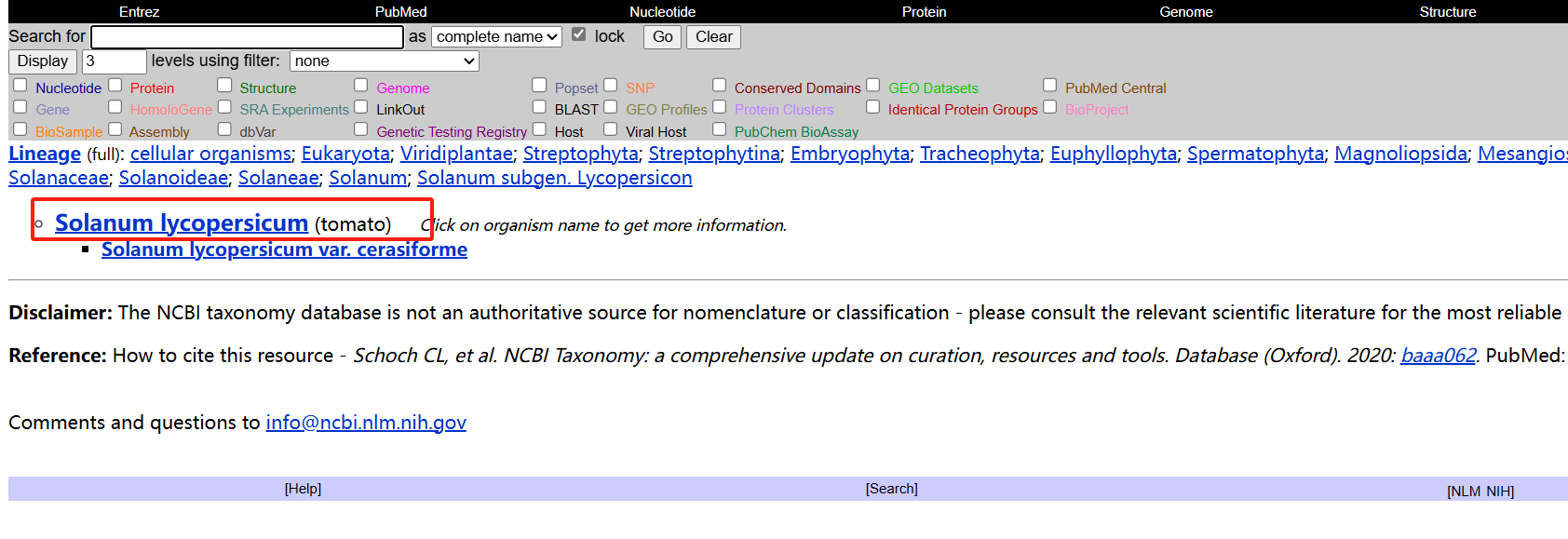
获得相关信息
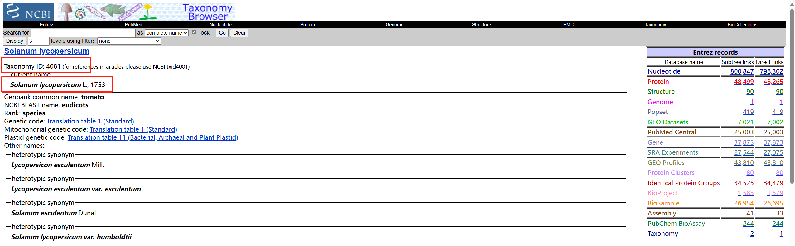
- 填写对应信息
tax_id="4081" genus="Solanum" species="lycompersicum" - 去重
gene2go <- unique(gene2go) gene2go <- gene2go[!duplicated(gene2go),] gene2ko <- gene2ko[!duplicated(gene2ko),] gene2pathway <- gene2pathway[!duplicated(gene2pathway),] - 构建OrgDb数据库
makeOrgPackage(gene_info=gene_info, go=gene2go, ko=gene2ko, pathway=gene2pathway, version="4.0", #版本 maintainer = "du<1678871583@qq.com>", #修改为你的名字和邮箱 author = "du<1678871583@qq.com>", #修改为你的名字和邮箱 outputDir = ".", #输出文件位置 tax_id=tax_id, genus=genus, species=species, goTable="go") 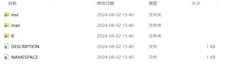
三、GO和KEGG富集分析
3.1 加载自建OrgDb数据库
install.packages("org.Slycompersicum.eg.db/", repos = NULL, type = "sources") 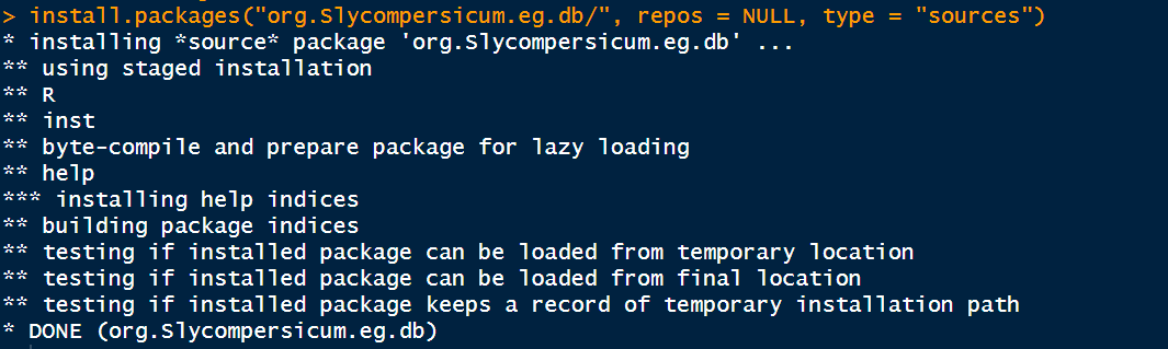
3.2 KEGG富集分析
- 读取DEG_list
DEG_list <- read.csv("DEG_list.csv",header = F) gene_list <- DEG_list$V1 - KEGG富集分析
pathway2gene <- AnnotationDbi::select(org.Slycompersicum.eg.db, keys = keys(org.Slycompersicum.eg.db), columns = c("Pathway","Ko")) %>% na.omit() %>% dplyr::select(Pathway, GID) - 导入 Pathway 与名称对应关系
load("kegg_info.RData") kegg <- enricher(gene_list, TERM2GENE = pathway2gene, TERM2NAME = pathway2name, pvalueCutoff = 1, qvalueCutoff = 1, pAdjustMethod = "BH", minGSSize = 200) - 查看KEGG富集结果
kegg_results <- as.data.frame(kegg) # head(kegg_results) ##'@导出结果 write.csv(kegg_results,"./KEGG_output.csv") 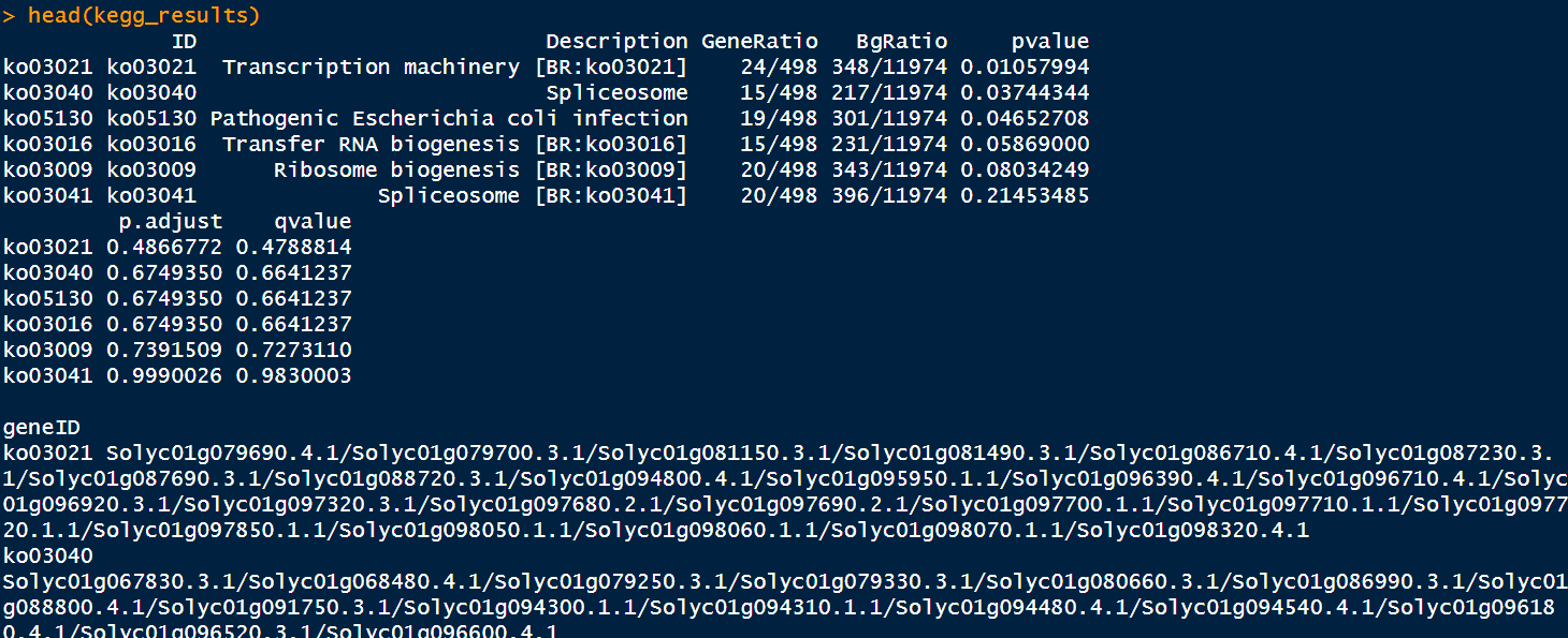
- 绘制柱状图
pdf("./功能富集/01.kegg.柱状图.pdf",height = 4, width = 6) barplot(kegg, showCategory= 10, drop=F, color="pvalue", font.size=10) dev.off() 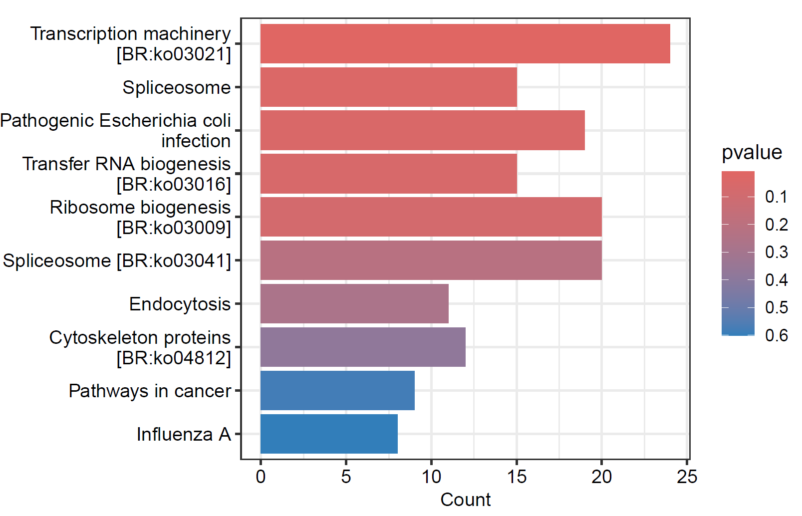
6. 气泡图
pdf("./功能富集/02.kegg.气泡图.pdf",height = 4, width = 6) dotplot(kegg) dev.off() 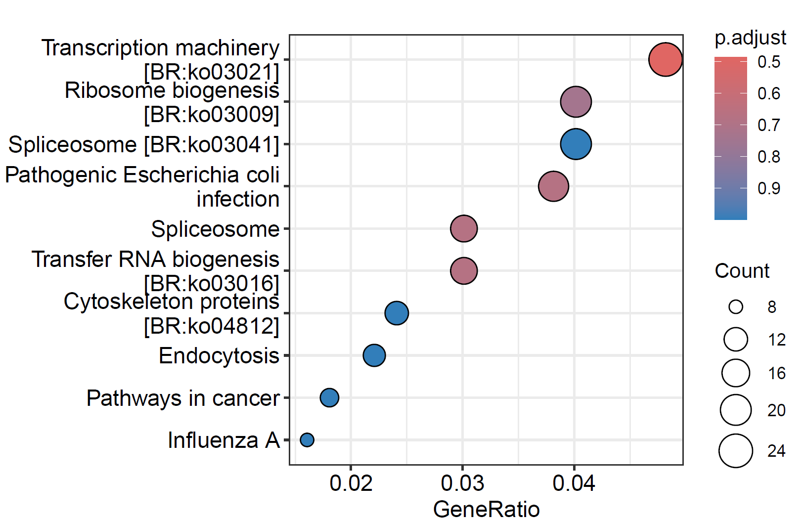
enrichplot::cnetplot(kegg,circular = F, colorEdge = T) 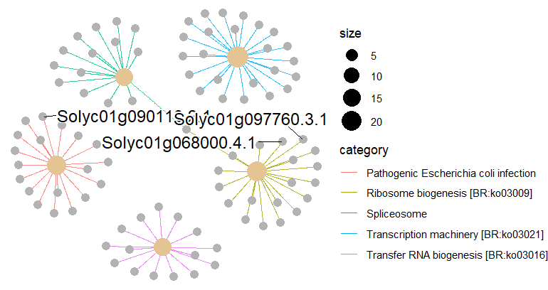
3.3 GO富集分析
enrich.go <- enrichGO(gene=gene_list, OrgDb = org.Slycompersicum.eg.db, # pvalueCutoff = 0.5, ##'@结合自己的需求进行调整 # qvalueCutoff = 0.5, ##'@结合自己的需求进行调整 pAdjustMethod = "BH", pvalueCutoff = 0.05, ont = "ALL", ## GO的种类,BP,CC, MF, ALL keyType = "GID") - 查看GO富集结果
GO_results <- as.data.frame(enrich.go) # head(GO_results) ##'@导出结果 write.csv(kegg_results,"./GO_output.csv") - 绘制GO富集柱状图
pdf(file = "./功能富集/03.GO_bar.pdf", width = 8, height = 6) barplot(enrich.go, drop = TRUE, showCategory = 10, ## 显示前10个GO term split="ONTOLOGY") + scale_y_discrete(labels=function(x) str_wrap(x, width=80))+ facet_grid(ONTOLOGY~., scale='free') dev.off() 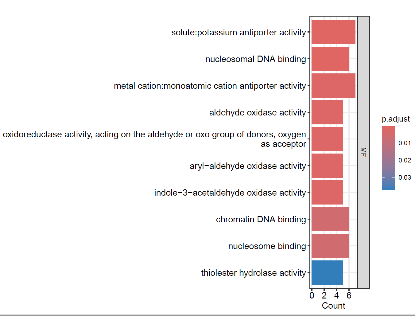
4. GO 气泡图
pdf(file = "./功能富集/04.GO_dotplot.pdf", width = 6, height = 6) dotplot(enrich.go, showCategory = 10) dev.off() - GO网络图
MF_ego <- enrichGO( gene = gene_list, keyType = "GID", OrgDb = org.Slycompersicum.eg.db, ont = "MF", ##'@GO的种类,BP,CC,MF pAdjustMethod = "BH", pvalueCutoff = 0.5 ##'@结合自己的需求进行调整 ) MF富集网络图
pdf("./功能富集/05.MF_网络图.pdf", width = 8, height = 8) plotGOgraph(MF_ego) dev.off() 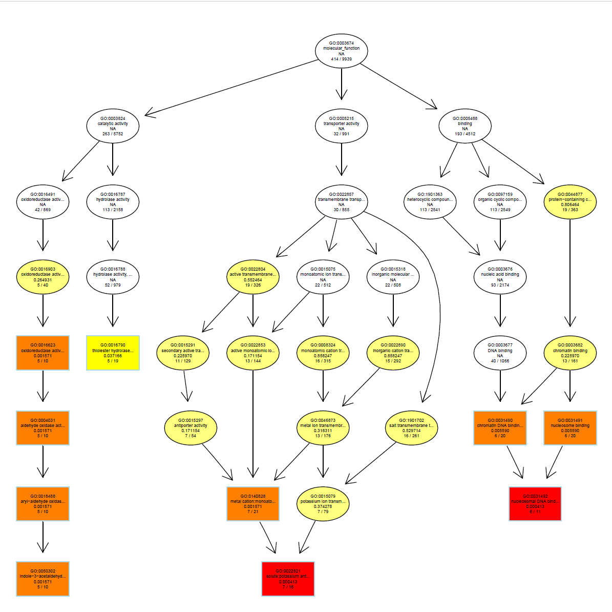
MF_ego <- pairwise_termsim(MF_ego) pdf("./功能富集/06.网络图.pdf",width = 8, height = 8) emapplot(MF_ego, cex.params = list(category_label = 0.8, line = 0.5)) + scale_fill_continuous(low = "#e06663", high = "#327eba", name = "p.adjust", guide = guide_colorbar(reverse = TRUE, order=2), trans='log10') dev.off() 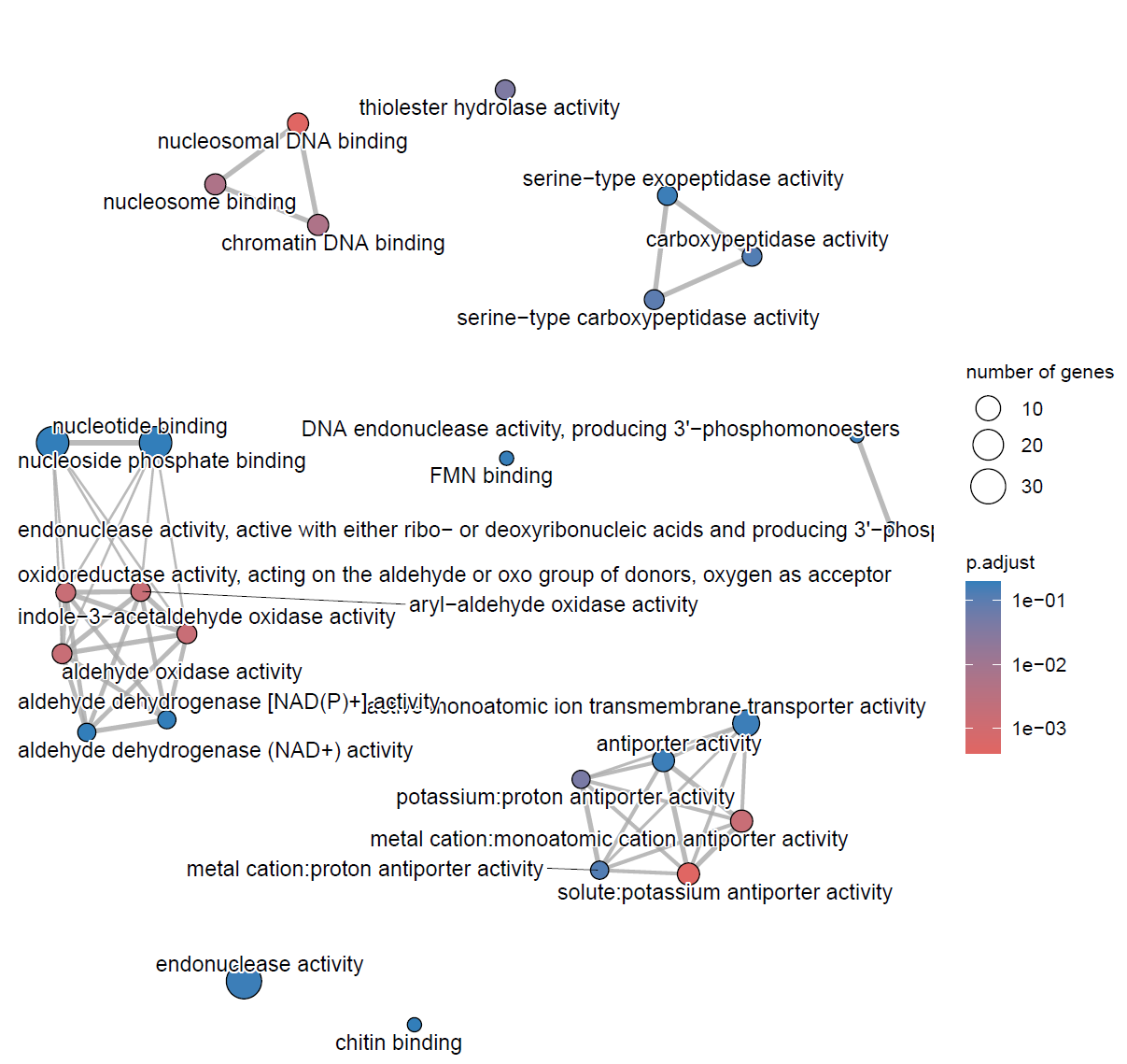
参考资源:
- https://www.jianshu.com/p/693d66681710
- https://www.jianshu.com/p/bb4281e6604e
- https://www.jianshu.com/p/9c9e97167377
- https://bioconductor.org/packages/release/bioc/vignettes/clusterProfiler/inst/doc/clusterProfiler.html#supported-organisms
若我们的教程对你有所帮助,请
点赞+收藏+转发,这是对我们最大的支持。
往期部分文章
1. 最全WGCNA教程(替换数据即可出全部结果与图形)
2. 精美图形绘制教程
3. 转录组分析教程
4. 转录组下游分析
小杜的生信筆記 ,主要发表或收录生物信息学教程,以及基于R分析和可视化(包括数据分析,图形绘制等);分享感兴趣的文献和学习资料!!
