
阅读量:0
Content
2.1 Import Necessary Libraries
Chapter 03 Descriptive Analysis
3.2 Dividing Features into Numerical or Categorical
3.3.2 Distribution of Categorical Variables
3.4.2 Distribution of Numerical Variables
3.5 Target Feature—HeartDisease
3.5.1 Categorical Features vs. Target Feature
3.5.2 Numerical Features vs. Target Feature
3.6 Relationships between Features
3.6.2 The Relationship between Sex, Age and Other Features
3.6.2.1 Sex, Age and RestingBP
3.6.2.2 Sex, Age and Cholesterol
4.1 Import Necessary Libraries
4.5 Linear Support Vector Machine
Chapter 01 Introduction
With a plethora of medical data available and the rise of Data Science, a host of startups are taking up the challenge of attempting to create indicators for the foreseen diseases that might be contracted! Cardiovascular diseases (CVDs) are the number 1 cause of death globally, taking an estimated 17.9 million lives each year, which accounts for 31% of all deaths worldwide. Heart failure is a common event caused by CVDs. People with cardiovascular disease or who are at high cardiovascular risk (due to the presence of one or more risk factors such as hypertension, diabetes, hyperlipidemia or already established disease) need early detection and management wherein a machine learning model can be of great help. With the help of AI techniques, we are able to classify / predict whether a patient is prone to heart failure depending on multiple attributes, thus providing reference for the diagnosis and treatment of heart disease.
The data used in this report is downloaded from Kaggle’s Heart Failure Prediction Dataset (Heart Failure Prediction Dataset | Kaggle). This dataset has created by combining different datasets already available independently but not combined before. In this dataset, 5 heart datasets are combined over 11 common features which makes it the largest heart disease dataset available so far for research purposes.
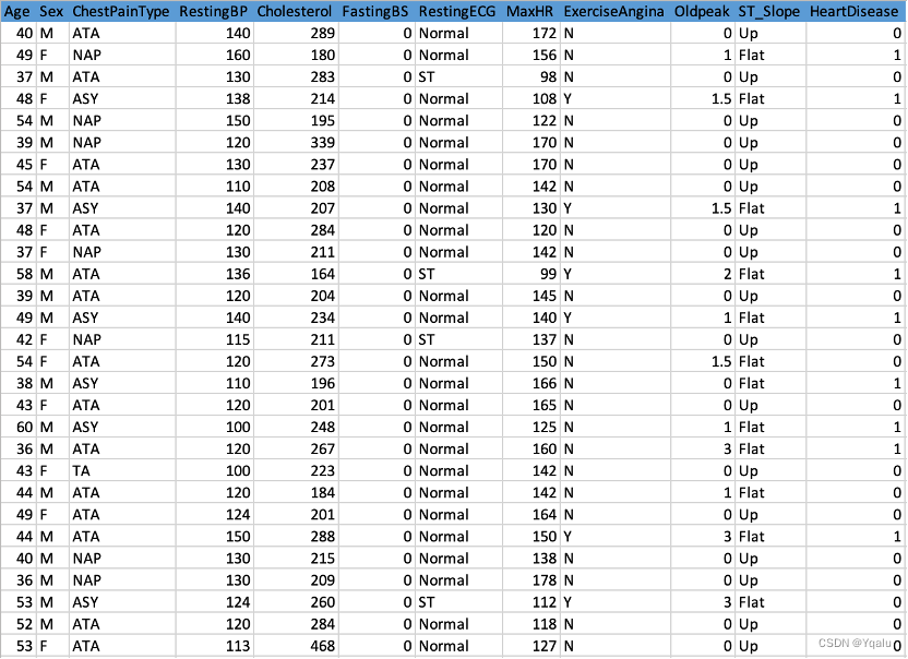
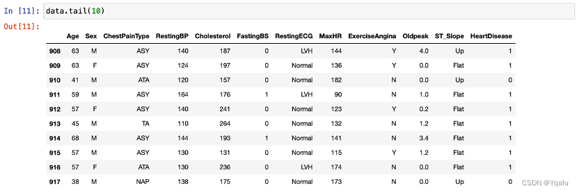
The indexes included in this dataset are Age, Sex, ChestPainType, RestingBP, Cholesterol, FastingBS, RestingECG, MaxHR, ExerciseAngina, Oldpeak, ST_Slope and HeartDisease.
To be more specific,
- Age: age of the patient [years]
- Sex : sex of the patient [M: Male, F: Female]
- ChestPainType : chest pain type [TA: Typical Angina, ATA: Atypical Angina, NAP: Non-Anginal Pain, ASY: Asymptomatic]
- RestingBP : resting blood pressure [mm Hg]
- Cholesterol : serum cholesterol [mm/dl]
- FastingBS : fasting blood sugar [1: if FastingBS > 120 mg/dl, 0: otherwise]
- RestingECG : resting electrocardiogram results [Normal: Normal, ST: having ST-T wave abnormality (T wave inversions and/or ST elevation or depression of > 0.05 mV), LVH: showing probable or definite left ventricular hypertrophy by Estes' criteria]
- MaxHR : maximum heart rate achieved [Numeric value between 60 and 202]
- ExerciseAngina : exercise-induced angina [Y: Yes, N: No]
- Oldpeak : oldpeak = ST [Numeric value measured in depression]
- ST_Slope : the slope of the peak exercise ST segment [Up: upsloping, Flat: flat, Down: downsloping]
- HeartDisease : output class [1: heart disease, 0: Normal]
In this report, the data will be first preprocessed by filling in missing values, substituting unusable variables and cleaning outliers. Then, we will focus on the descriptive characteristics of data through visual diagrams. After that, training set and the test set will be divided and the Decision Tree model will be built and modified. Finally, we will look into alternative models to fully evaluate the effectiveness of prediction. Based on the models, conclusions will be made and further research suggestion will also be given.
Chapter 02 Preparation
2.1 Import Necessary Libraries
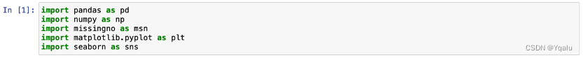
- Pandas: Pandas is a library in Python that provides data structures and tools for data analysis. It offers a DataFrame, a table-like structure that can store and manipulate large amounts of data efficiently. Pandas provides capabilities like data indexing, filtering, merging, and much more. It's the backbone of many data analysis projects in Python.
- Numpy: Numpy is a library that provides support for large, multi-dimensional arrays and matrices. It is the core library for numerical computations in Python. Numpy's arrays are highly optimized for speed and come with a large set of mathematical functions, such as linear algebra, statistics, and Fourier transform.
- Matplotlib: Matplotlib is a Python 2D plotting library that produces publication-quality figures. It offers a wide range of plotting options, from simple line graphs to complex bar charts, scatter plots, and more. Matplotlib is often used in combination with other libraries like Pandas and Numpy to enhance data visualization.
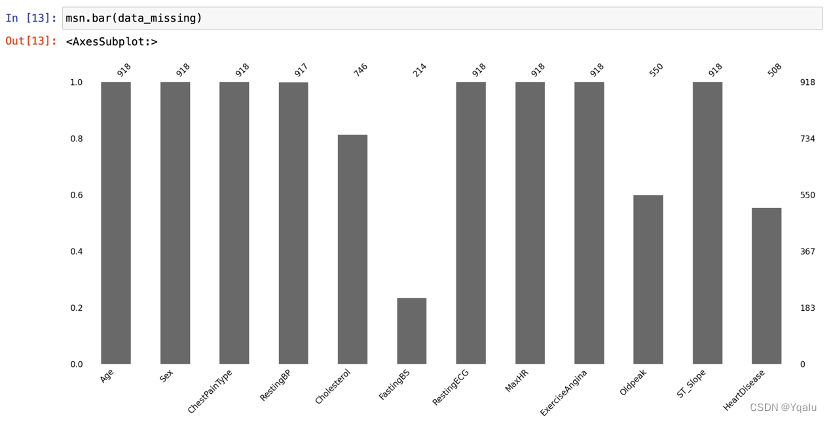
- Missingno: Missingno is a Python library that helps in handling missing data in DataFrame-like structures. It provides visualizations to understand missing data patterns and suggests imputation methods to fill in the missing values. Missingno is a valuable tool for data exploration and cleaning.
- Seaborn: Seaborn is a Python data visualization library built on top of Matplotlib. It leverages the power of Matplotlib but provides a higher-level interface for creating statistical graphics. Seaborn's designs are based on the grammar of graphics, making it easy to create complex visualizations with just a few lines of code.
2.2 Import Dataset
![]()
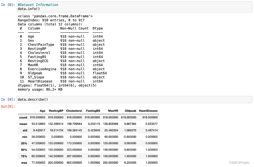
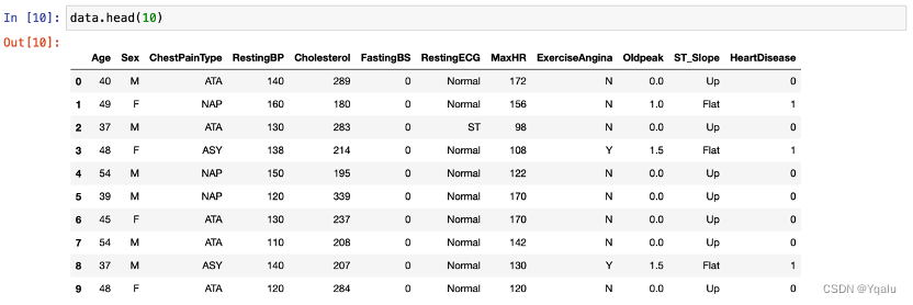
2.3 Check Basic Information
Check the dataset information by calling functions such as:
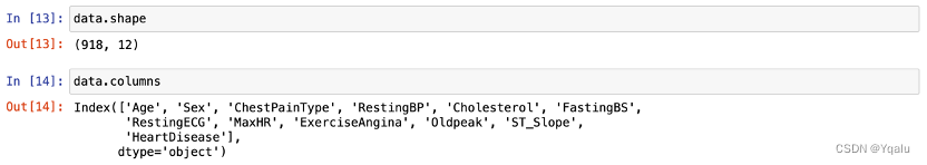
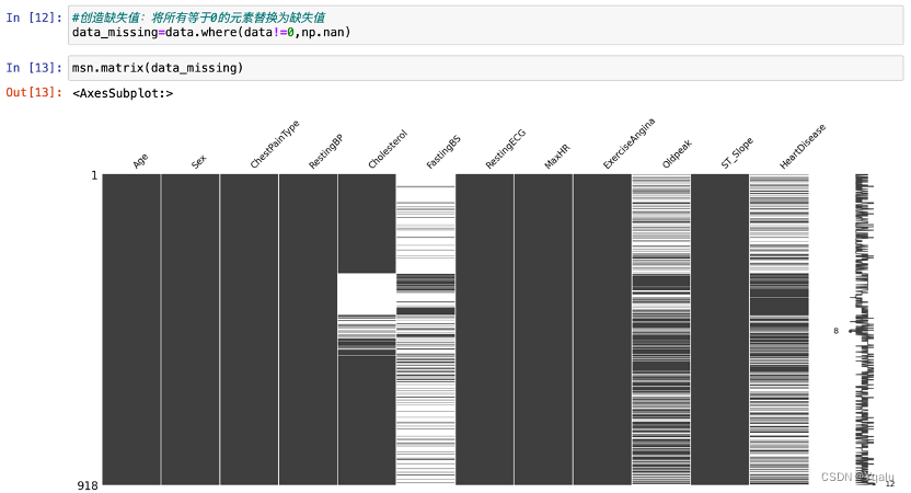
2.4 Check Missing Values
Check the missing values by calling functions such as:
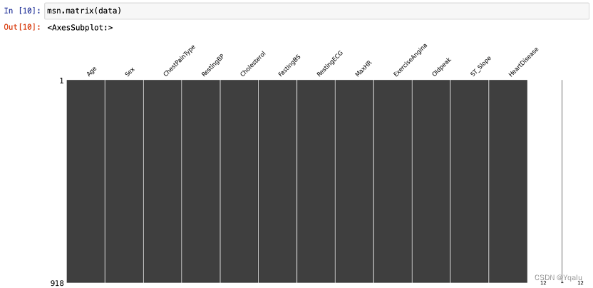
Apparently, the dataset has 918 rows and 12 columns, with no missing values overall. As a trial, this report will replace all data with values of 0 by missing values, in order to better demonstrate the effects of a dataset with missing values as well as the use of missingno library.
Chapter 03 Descriptive Analysis
3.1 Overview
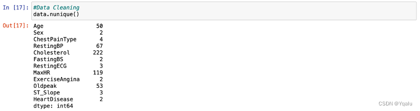
Check the unique values in every feature by calling the function:
3.2 Dividing Features into Numerical or Categorical
Distinguish categorical features and numerical features by the number of unique values included. If the number of unique values of certain feature is greater than six, this feature will be treated as numerical feature. Otherwise, it will be treated as categorical features.
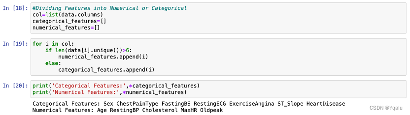
According to the output, seven features —— “Sex”, “ChestPainType”, “FastingBS”, “RestingECG”, “ExerciseAngina”, “ST_Slope” and “HeartDisease” —— belong to categorical features, and five features —— “Age”, “RestingBP”, “Cholesterol”, “MaxHR” and “Oldpeak” —— belong to numerical features.
3.3 Categorical Features
3.3.1 Mapping
In order to simplify later analysis and modeling, this report will first assign string classifiers to 0,1,2,3, … numeric classifiers. The steps are as follows.
Method.1
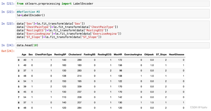
LabelEncoder is a library in Python that is often used for encoding categorical variables. It converts categorical labels into numerical values that can be used for further analysis or machine learning tasks.
Method.2
For this dataset, as the number of features is less, we are also able to convert string classifiers into numerical classifiers by manual assignment, which makes the mapping result more controllable.
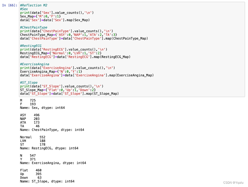
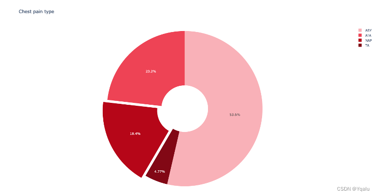
Take the ChestPainType as an example. value_counts() function is used to obtain the frequency of each value and the result shows that there are four values in ChestPainType, which is “ASY”, “NAP”, “ATA”, and “TA”. Then, we can build a mapping dictionary to replace the original data with 0, 1, 2 and 3. Other features are similarly mapped.
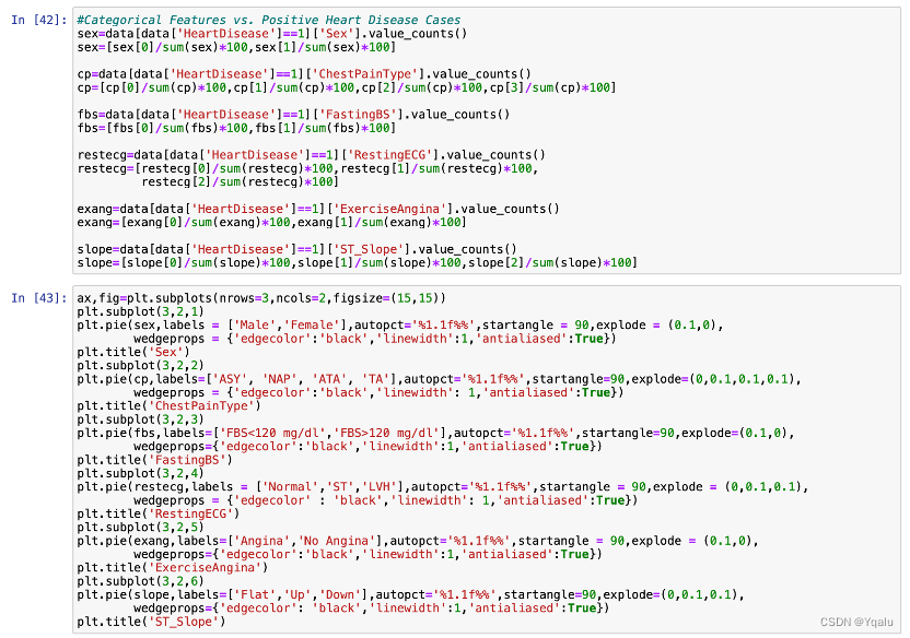
3.3.2 Distribution of Categorical Variables
After mapping the data, we will now examine the distribution of those categorical variables.
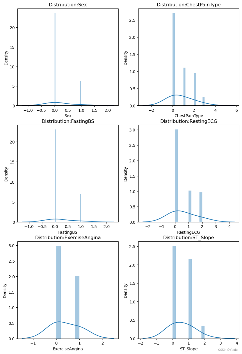

As shown in the graphs,
- Sex [M, F]: The sample size of males are approximately three times as large as the females’ sample size.
- ChestPainType [ASY, NAP, ATA, TA]: The sample size of NAP and ATA is similar, and ASY is about 2.5 times and TA is about ¼.
- FastingBS [0, 1]: The number of samples equal to 0 are nearly three times the sample size of 1.
- RestingECG [Normal, LVH, ST]: 60% of the data is Normal, with LVH and ST each accounting for the another 20%.
- ExerciseAngina [N, Y]: N is 1.5 times Y.
- ST_Slope [Flat, Up, Down]: Flat makes up half of the sample size, Up 40% and Down less than 10%.
3.4 Numerical Features
3.4.1 Data Cleaning
The outliers of continuous variables also need to be excluded.
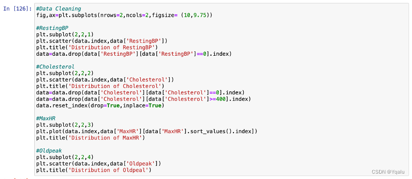

Take the RestingBP and Cholesterol as examples. According to the actual situation, the RestingBP could not be 0. Considering the relatively small number of outliers, this report deletes the outlier directly by calling the “drop” function. Similarly, Cholesterol values greater than 400 or equal to 0 are also considered outliers and excluded.
3.4.2 Distribution of Numerical Variables
After cleaning the data, we will now examine the distribution of those numerical variables to check the basic structure of dataset.
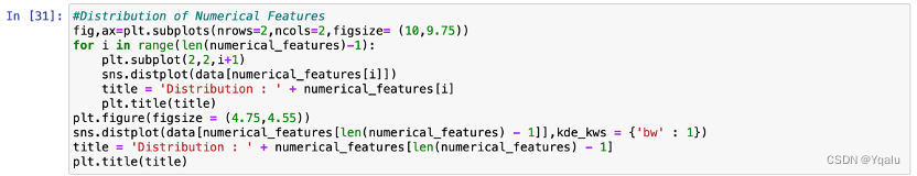
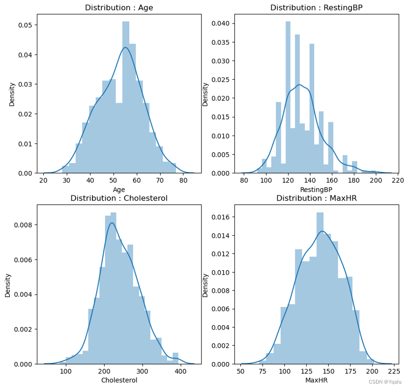

All features are approximately normally distributed except Oldpeak, which seems to be right-skewed.
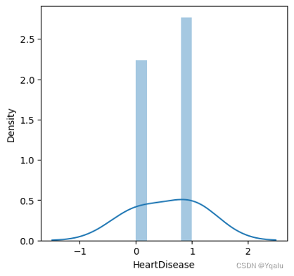
3.5 Target Feature—HeartDisease
After cleaning the data, we will focus on the target feature, which is, HeartDisease.
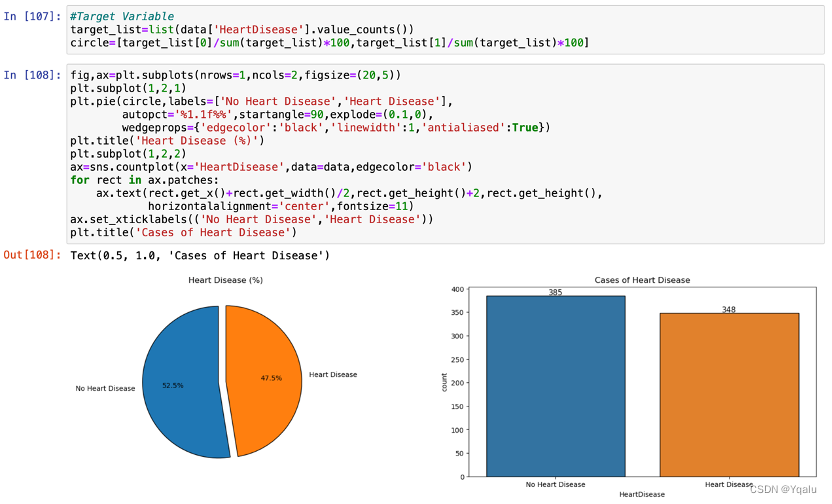
The dataset is pretty evenly balanced. There are 385 samples which are free of heart disease, accounting for 52.5% of the total samples while 348 people are diagnosed with heart disease, accounting for 47.5%.
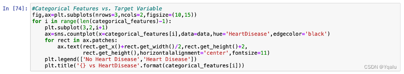
3.5.1 Categorical Features vs. Target Feature
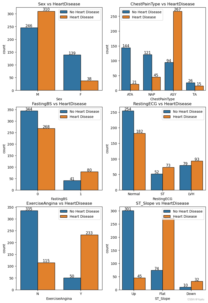
- Male population has more heart disease patients than no heart disease patients. In the case of Female population, heart disease patients are less than no heart disease patients.
- ASY type of chest pain boldly points towards major chances of heart disease.
- Patients diagnosed with Fasting Blood Sugar and no Fasting Blood Sugar have significant heart disease patients.
- RestingECG does not present with a clear-cut category that highlights heart disease patients. All the 3 values consist of high number of heart disease patients.
- Exercise Induced Engina definitely bumps the probability of being diagnosed with heart diseases.
- With the ST_Slope values, flat slope displays a very high probability of being diagnosed with heart disease. Down also shows the same output but in very few data points.
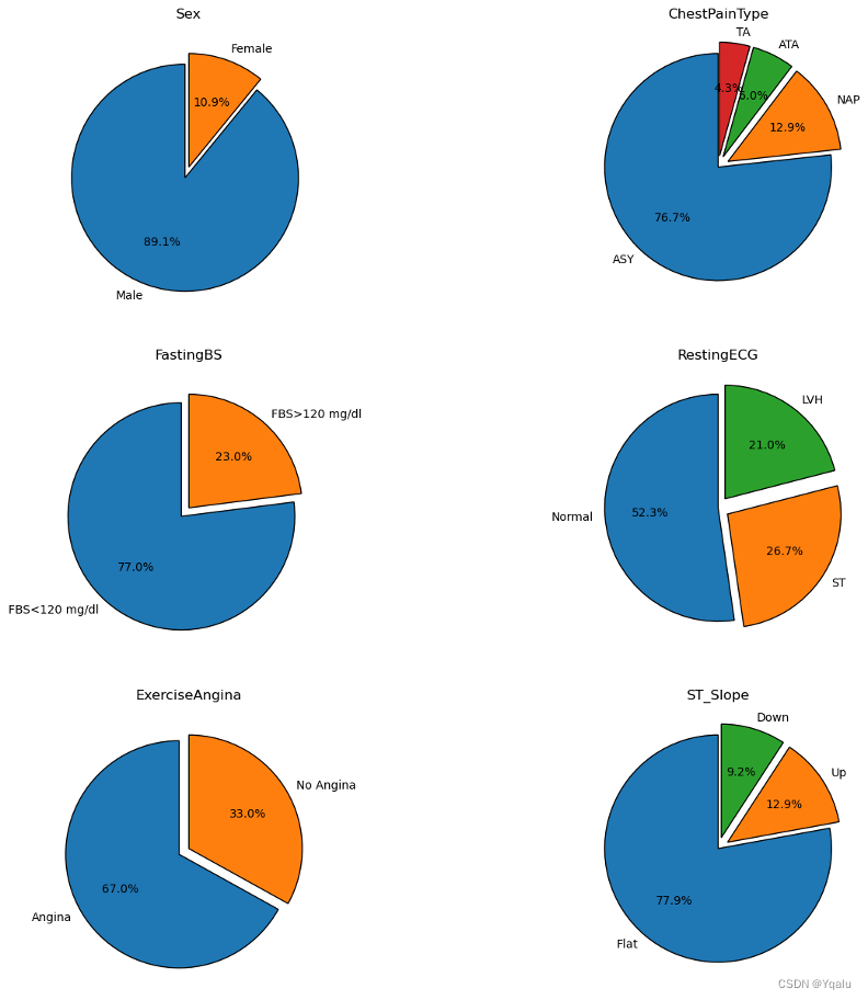
- Out of all the heart disease patients, a staggering 90% patients are male.
- When it comes to the type of chest pain, ASY type holds the majority with 77% that lead to heart diseases.
- Fasting Blood Sugar level < 120 mg/dl displays high chances of heart diseases.
- For RestingECG, Normal level accounts for 56% chances of heart diseases than LVH and ST levels.
- Detection of Exercise Induced Angina also points towards heart diseases.
- When it comes to ST_Slope readings, Flat level holds a massive chunk with 75% that may assist in detecting underlying heart problems.
3.5.2 Numerical Features vs. Target Feature
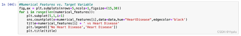
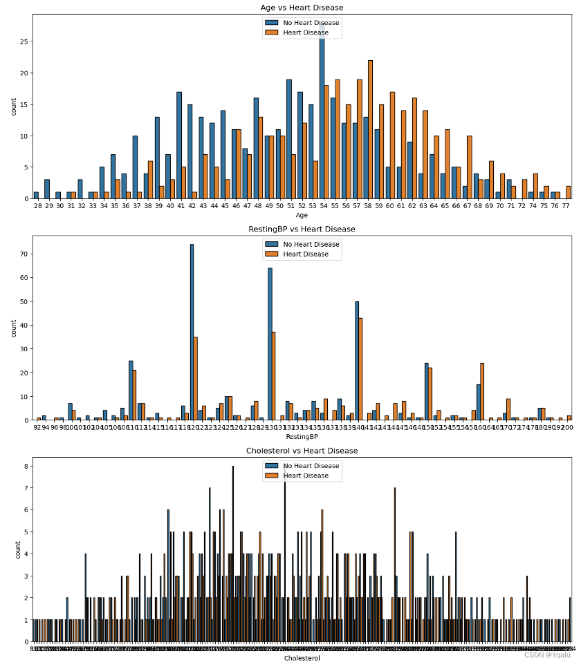

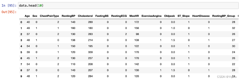
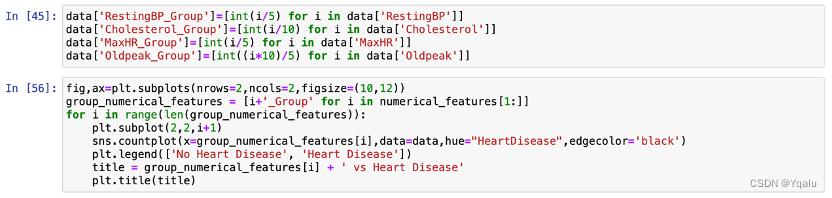
Because of too many unique data points in the above features, it is difficult to gain any type of insight. Thus, we will convert these numerical features,except age, into categorical features for understandable visualization and gaining insights purposes.
Thus, we scale the individual values of these features. This brings the varied data points to a constant value that represents a range of values.
Here, we divide the data points of the numerical features by 5 or 10 and assign its quotient value as the representative constant for that data point. The scaling constants of 5 and 10 are decided by looking into the data & intuition.

From the RestingBP group data, 95 (19x5) - 170 (34x5) readings are most prone to be detected with heart diseases.
Cholesterol levels between 160 (16x10) - 340 (34x10) are highly susceptible to heart diseases.
For the MaxHR readings, heart diseases are found throughout the data but 70 (14x5) - 180 (36x5) values has detected many cases.
Oldpeak values also display heart diseases throughout. 0 (0x5/10) - 4 (8x5/10) slope values display high probability to be diagnosed with heart diseases.
3.6 Relationships between Features
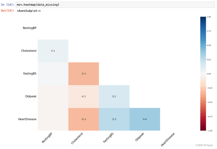
3.6.1 Correlation
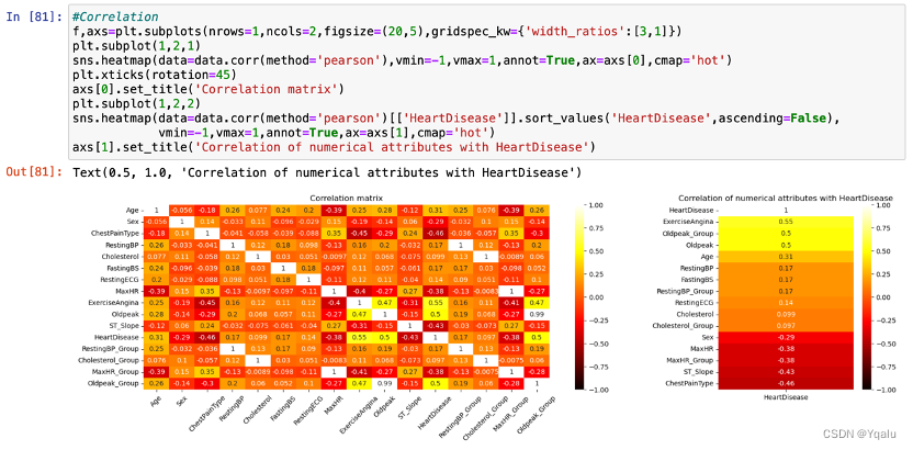
All features display a positive or negative relationship with HeartDisease.
![]()

3.6.2 The Relationship between Sex, Age and Other Features
3.6.2.1 Sex, Age and RestingBP
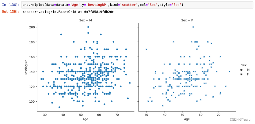
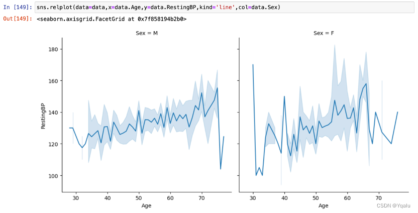
With the increase of age, the RestingBP also shows an increasing trend. Besides, the RestingBP of women in the same age group is slightly lower than that of man.
3.6.2.2 Sex, Age and Cholesterol
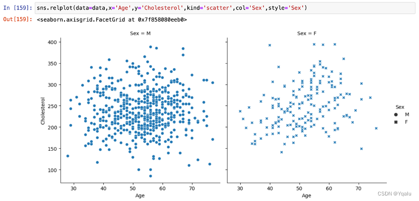
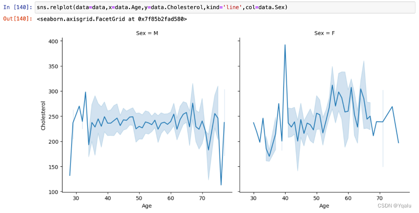
The data of Cholersterol also tends to increase with age, but there seems to be a turning point around the age of 70, and after that, Cholersterol becomes a decline with age. In addition, Cholesterol in women of the same age appeared to be more discrete and varied between individuals, in comparison with men.
3.6.2.3 Sex, Age and MaxHR
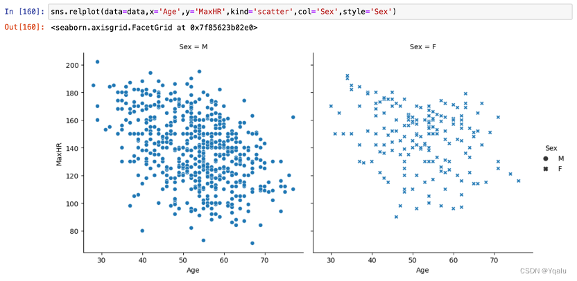
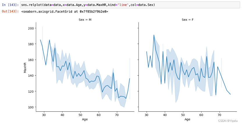
MaxHR showed an obvious decreasing trend with age. In terms of gender comparison, the rate of decline was lower in women than in men.
3.6.2.4 Sex, Age and Oldpeak
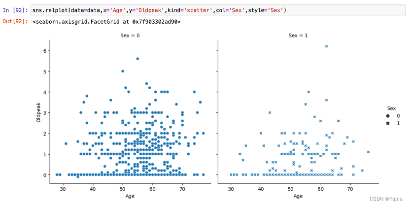
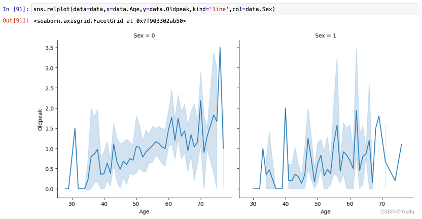
Oldpeak slightly showed an upward trend with the increase of age, and the increasing trend of female is lower than that of male.
Chapter 04 Model
4.1 Import Necessary Libraries
from sklearn.model_selection import train_test_split from sklearn.metrics import confusion_matrix,accuracy_score from sklearn.linear_model import LogisticRegression from sklearn.neighbors import KNeighborsClassifier from sklearn.svm import SVC from sklearn.naive_bayes import GaussianNB from sklearn.tree import export_graphviz from sklearn.model_selection import GridSearchCV from sklearn.preprocessing import MinMaxScaler,StandardScaler import graphviz from sklearn.ensemble import RandomForestClassifier- Sklearn: Scikit-learn (sklearn) is a popular Python library that provides a wide range of tools for data analysis, data exploration, and machine learning. It is a key component of the scikit-family of libraries, which are built on NumPy, SciPy, and matplotlib.
- Graphviz: Graphviz is a graph visualization software package that can generate static and interactive graphs. It is widely used in various fields, including data science, software engineering, and network analysis.
4.2 Decision Tree
Decision Tree is a popular machine learning algorithm that belongs to the family of classification models. It is widely used in various applications such as customer segmentation, credit risk assessment, and medical diagnosis.
Decision Tree works by recursively splitting the data based on the best split criterion. It starts with a root node that contains the entire dataset and then recursively splits the data into smaller and smaller subsets. The split criterion is determined by a specific metric such as information gain or Gini impurity. The process of splitting continues until a stopping criterion is met, such as when a node becomes pure or a maximum depth is reached.
The key advantage of Decision Tree is its ability to handle both numerical and categorical data, as well as its simplicity and ease of understanding. It provides an intuitive representation of the decision process and can easily be interpreted by domain experts. Decision Tree also has a built-in feature selection mechanism that identifies the most important features in the data, which can be used for model building and optimization.
4.2.1 Preparation
Machine learning model does not understand the units of the values of the features. It treats the input just as a simple number but does not understand the true meaning of that value. Thus, it becomes necessary to scale the data.
We have 2 options for data scaling :
- Normalization
- Standardization
As most of the algorithms assume the data to be normally (Gaussian) distributed, Normalization is done for features whose data does not display normal distribution and standardization is carried out for features that are normally distributed where their values are huge or very small as compared to other features.
- Normalization : According to the previous descriptive analysis, we find that Oldpeak might be right-skewed. Therefore, Oldpeak feature is first examined, and then normalized if it had confirmed to be right-skewed.
- Standardizarion : Age, RestingBP, Cholesterol and MaxHR features are scaled down because these features are normally distributed.
Method.1
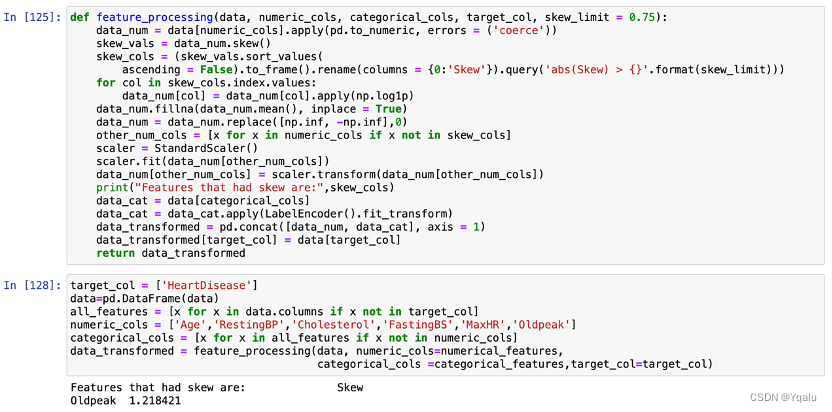
The result confirms our hypothesis that Oldpeak is, indeed, right-skewed while other features fit the normal distribution.
Method.2
By using MinMaxScaler and StandardScaler, the computer can process the data for us automatically.
mms = MinMaxScaler() ss = StandardScaler() data['Oldpeak'] = mms.fit_transform(data[['Oldpeak']]) data['Age'] = ss.fit_transform(data[['Age']]) data['RestingBP'] = ss.fit_transform(data[['RestingBP']]) data['Cholesterol'] = ss.fit_transform(data[['Cholesterol']]) data['MaxHR'] = ss.fit_transform(data[['MaxHR']])4.2.2 Split
Split the data set into 80% of the experimental data set and 20% of the test data set.
target=np.array(data['HeartDisease']) data=np.array(data.drop('HeartDisease',axis=1)) Xtrain,Xtest,Ytrain,Ytest=train_test_split(data,target,test_size=0.2,random_state=0) print('Shape of training feature:',Xtrain.shape) print('Shape of testing feature:',Xtest.shape) print('Shape of training label:',Ytrain.shape) print('Shape of testing label:',Ytest.shape)Output:
Shape of training feature: (581, 11)
Shape of testing feature: (146, 11)
Shape of training label: (581,)
Shape of testing label: (146,)
The training set includes 581 samples and the testing set 146 samples.
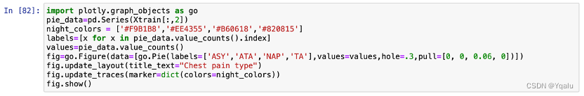
Check the distribution of ChestPainType in Xtrain by using pie chart:
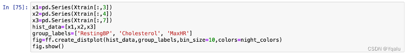
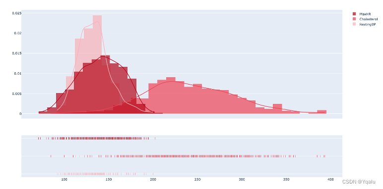
Check the distribution of MaxHR, Cholesterol and RestingBP by using hist graph:
4.2.3 Fit
clf_1=tree.DecisionTreeClassifier() clf_1=clf_1.fit(Xtest,Ytest) score=clf_1.score(Xtest,Ytest) print(score)Output:
1.0
It is very high that the accuracy of the fitted model reaches 100%. Next, we look at how important each feature is.
feature_name=['Age','Sex','ChestPainType','RestingBP','Cholesterol','FastingBS','RestingECG','MaxHR','ExerciseAngina','Oldpeak','ST_Slope'] print([*zip(feature_name,clf.feature_importances_)])Output:
[('Age', 0.03902032246974199),
('Sex', 0.10413167080271438),
('ChestPainType', 0.03755102040816328),
('RestingBP', 0.047895421178778846),
('Cholesterol', 0.13245268588124812),
('FastingBS', 0.05597883597883598),
('RestingECG', 0.0),
('MaxHR', 0.03763852588484448),
('ExerciseAngina', 0.16062716853917341),
('Oldpeak', 0.029206349206349205),
('ST_Slope', 0.3554979996501504)]
The feature ST_Slope is very important, accounting for more than 0.3.
4.2.4 The 1st Decision Tree
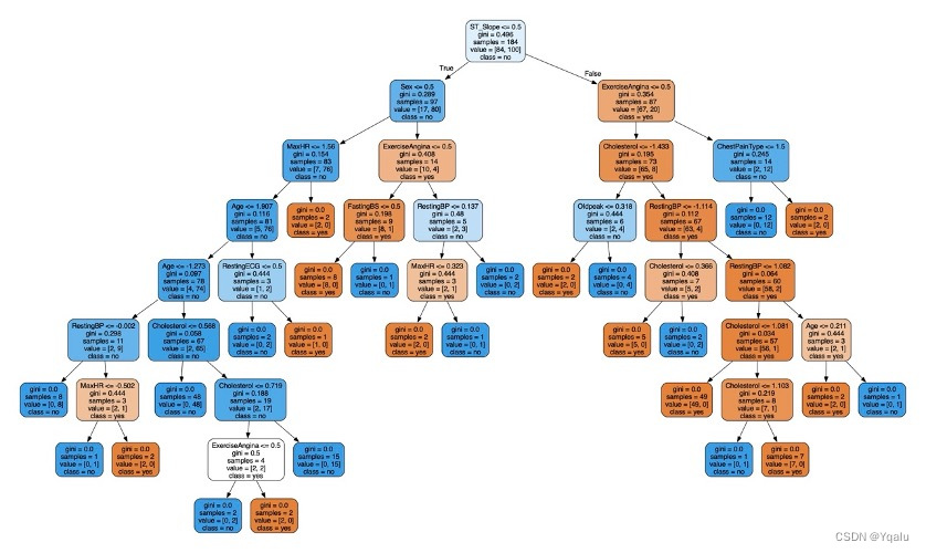
In this visualization part, we import graphviz package and build the first Decision Tree model. The parameters are clf (classifier), feature_names (column names), class_name (category label name), filled (color filled), and rounded (rounded).
dot_data=export_graphviz(clf_1,out_file=None,feature_names=feature_name,class_names=['yes','no'],filled=True,rounded=True) graph=graphviz.Source(dot_data) graph.render(filename='Decision_tree_1',directory='/Users/luyiwei/Desktop',view=True)Output:
Ypred=clf_1.predict(Xtest) cm=confusion_matrix(Ytest,Ypred) tree_train_acc=round(accuracy_score(Ytrain,clf_1.predict(Xtrain))*100,2) tree_test_acc=round(accuracy_score(Ytest,Ypred)*100,2) print('Accuracy (Decision Tree)=',tree_test_acc,'%') print('The Mean Absolute Error (Decision Tree)=',round(mean_absolute_error(Ytest,Ypred),2)) print('Classification Report (Decision Tree)=\n',classification_report(Ytest,Ypred)) sns.heatmap(cm,annot=True,fmt='d',cmap='Blues',cbar=False) plt.title('Decision Tree Confusion Matrix') plt.show()Output:
Accuracy (Decision Tree)= 100.0 %
The Mean Absolute Error (Decision Tree)= 0.0
The prediction accuracy of this model is as high as 100%, so it is an over-fitting model, which will lead to poor generalization ability and need to be optimized.
4.2.5 Optimize
When building the model, that is, a classifier, there are a large number of parameters that can be adjusted. For example:
clf=tree.DecisionTreeClassifier(criterion=’gini’, max_depth=4, max_leaf_nodes=10, min_samples_leaf=9)The setting of parameters can improve the accuracy and generalization ability of the model. We import GridSearchCV. Parameter alternatives form a dictionary, such as' criterion ':[' gini', 'entropy'], with alternatives as' gini 'and' entropy '. The GridSearchCV parameter includes clf (model), parameters (parameter), refit (whether the training set is cross-validated), cv (cross-validated parameter), verbose (log verbose, int: verbose, 0: no training process output, 1: occasional output, > 1: output for each submodel), n_jobs (-1 stands for multi-core).
Xtrain,Xtest,Ytrain,Ytest=train_test_split(data,target,test_size=0.3,random_state=0) clf_2=tree.DecisionTreeClassifier() parameters={'max_depth':[1,2,3,4,5,6,7,8,9], 'max_leaf_nodes':range(20), 'criterion':['gini','entropy'], 'min_samples_leaf':range(15)} gs=GridSearchCV(clf_2,parameters,refit=True,cv=5,verbose=1,n_jobs=-1) gs.fit(Xtrain,Ytrain) print(gs.best_score_) print(gs.best_params_)Output:
0.8485509272202032
{'criterion': 'gini', 'max_depth': 8, 'max_leaf_nodes': 17, 'min_samples_leaf': 5}
Optimized model is set according to the optimal parameters above.
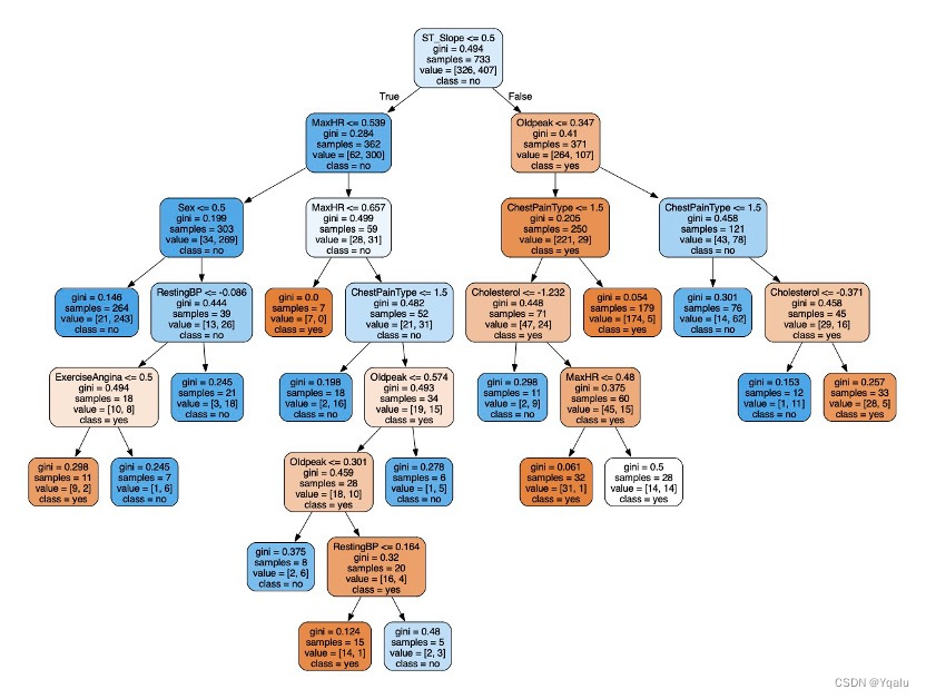
clf_2=tree.DecisionTreeClassifier(criterion='gini',max_depth=8,max_leaf_nodes=17,min_samples_leaf=5) clf_2=clf_2.fit(Xtrain,Ytrain) score=clf_2.score(Xtest,Ytest) dot_data=tree.export_graphviz(clf_2,out_file=None,feature_names=feature_name,class_names=['yes','no'],filled=True,rounded=True) graph=graphviz.Source(dot_data) graph.render(filename='Decision_tree_2',directory='/Users/luyiwei/Desktop',view=True)Output:

4.2.6 Verify
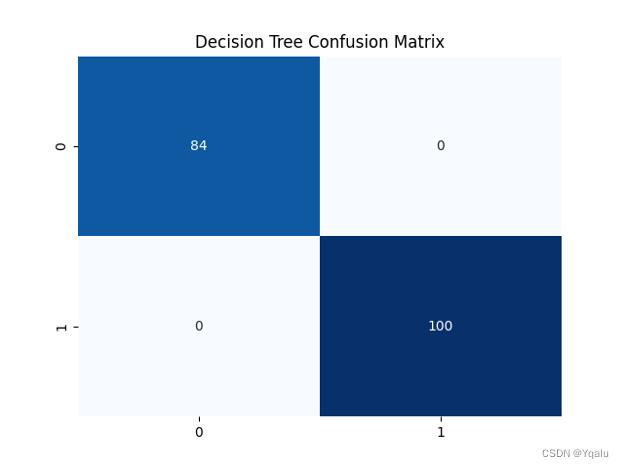
Ypred=clf_2.predict(Xtest) cm=confusion_matrix(Ytest,Ypred) tree_train_acc=round(accuracy_score(Ytrain,clf_2.predict(Xtrain))*100,2) tree_test_acc=round(accuracy_score(Ytest,Ypred)*100,2) print('Accuracy (Decision Tree)=',tree_test_acc,'%') print('The Mean Absolute Error (Decision Tree)=',round(mean_absolute_error(Ytest,Ypred),2)) print('Classification Report (Decision Tree)=\n',classification_report(Ytest,Ypred)) sns.heatmap(cm,annot=True,fmt='d',cmap='Blues',cbar=False) plt.title('Decision Tree Confusion Matrix') plt.show()Output:
Accuracy (Decision Tree)= 89.67 %
The Mean Absolute Error (Decision Tree)= 0.1

4.3 Logistic Regression
Logistic Regression assumes that the target variable follows a binary distribution, such as Bernoulli or binomial. It models the relationship between the input features and the target variable using a logistic function. The logistic function takes the linear combination of the input features and the corresponding weights as input and returns the probability of the target variable being in the positive class.
The Logistic Regression model is trained by minimizing a loss function that measures the difference between the predicted probabilities and the true labels. The most common loss function used in Logistic Regression is the binary cross-entropy loss.
The key advantage of Logistic Regression is its simplicity and ease of understanding. It provides a linear model for binary classification tasks and can be easily interpreted. Logistic Regression also has good computational efficiency and can be trained using gradient descent or other optimization algorithms.
lr=LogisticRegression() lr.fit(Xtrain,Ytrain) Ypred=lr.predict(Xtest) cm=confusion_matrix(Ytest,Ypred) lr_train_acc=round(accuracy_score(Ytrain,lr.predict(Xtrain))*100,2) lr_test_acc=round(accuracy_score(Ytest,Ypred)*100,2) print('Accuracy (Logistic Regression)=',lr_test_acc,'%') print('The Mean Absolute Error (Logistic Regression)=',round(mean_absolute_error(Ytest,Ypred),2)) print('Classification Report (Logistic Regression)=\n',classification_report(Ytest,Ypred)) sns.heatmap(cm,annot=True,fmt='d',cmap='Blues',cbar=False) plt.title('Logistic Regression Confusion Matrix') plt.show()Output:
Accuracy (Logistic Regression)= 87.5 %
The Mean Absolute Error (Logistic Regression)= 0.12

4.4 K-Nearest Neighbors
The K-Nearest Neighbors (KNN) model is a fundamental and widely used machine learning algorithm. It belongs to the category of instance-based learning methods, where the prediction of a new data point is based on the similarity of that data point to other known data points in the training set.
In the KNN algorithm, the similarity between data points is measured using a distance metric, such as Euclidean distance or Manhattan distance. The algorithm selects the k nearest neighbors of the query data point based on this distance metric and uses their class labels to make a prediction.
The prediction is typically done by majority voting or weighted voting, where the class labels of the k nearest neighbors are considered and the most frequent class label is assigned to the query data point.
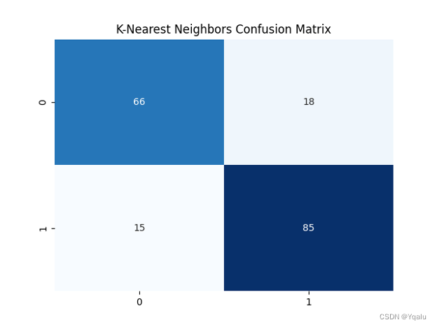
knn=KNeighborsClassifier(n_neighbors=3) knn.fit(Xtrain,Ytrain) Ypred=knn.predict(Xtest) cm=confusion_matrix(Ytest, Ypred) knn_train_acc=round(accuracy_score(Ytrain,knn.predict(Xtrain))*100,2) knn_test_acc=round(accuracy_score(Ytest,Ypred)*100,2) print('Accuracy (K-Nearest Neighbors)=',knn_test_acc,'%') print('The Mean Absolute Error (K-Nearest Neighbors)=',round(mean_absolute_error(Ytest,Ypred),2)) print('Classification Report (K-Nearest Neighbors)=\n',classification_report(Ytest,Ypred)) sns.heatmap(cm,annot=True,fmt='d',cmap='Blues',cbar=False,) plt.title('K-Nearest Neighbors Confusion Matrix') plt.show()Output:
Accuracy (K-Nearest Neighbors)= 82.07 %
The Mean Absolute Error (K-Nearest Neighbors)= 0.18
4.5 Linear Support Vector Machine
The linear support vector machine (SVM) model is a fundamental and widely used machine learning algorithm in the field of classification and regression analysis. It belongs to the family of kernel-based methods, where the key idea is to transform the input data into a higher-dimensional feature space using a kernel function.
In the linear SVM, the transformed feature space is spanned by a set of support vectors that are selected to separate the classes in the feature space. The separating hyperplane is determined by the support vectors and their associated weights.
svm=SVC(kernel='linear') svm.fit(Xtrain,Ytrain) Ypred = svm.predict(Xtest) cm=confusion_matrix(Ytest, Ypred) svm_train_acc=round(accuracy_score(Ytrain,svm.predict(Xtrain))*100,2) svm_test_acc=round(accuracy_score(Ytest,Ypred)*100,2) print('Accuracy (Linear Support Vector Machine)=',svm_test_acc,'%') print('The Mean Absolute Error (Linear Support Vector Machine)=', round(mean_absolute_error(Ytest,Ypred),2)) print('Classification Report (Linear Support Vector Machine)=\n', classification_report(Ytest,Ypred)) sns.heatmap(cm,annot=True,fmt='d',cmap='Blues',cbar=False,) plt.title('Support Vector Machine Confusion Matrix') plt.show()Output:
Accuracy (Linear Support Vector Machine)= 89.13 %
The Mean Absolute Error (Linear Support Vector Machine)= 0.11

4.6 Kernel Support Vector Machine
Kernel Support Vector Machine (SVM) is a machine learning model that belongs to the family of kernel methods. It is a powerful tool for pattern recognition and classification tasks, particularly in high-dimensional or nonlinear data spaces.
Kernel SVM works by mapping the input data into a higher-dimensional feature space using a kernel function. This mapping is done implicitly, without explicitly calculating the new feature vectors. The mapped data then resides in a feature space where the separation between classes is maximized, leading to better classification performance.
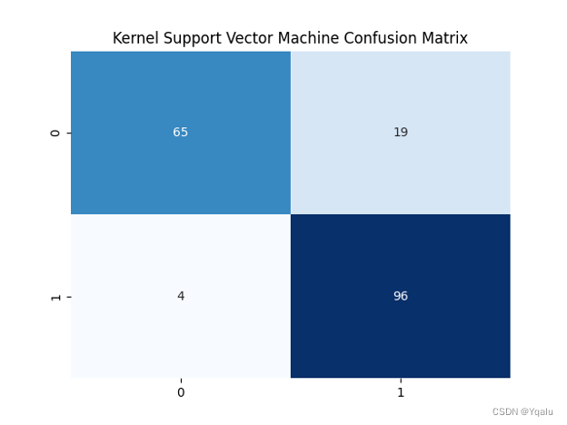
svm_kernel=SVC(kernel='rbf') svm_kernel.fit(Xtrain,Ytrain) Ypred = svm_kernel.predict(Xtest) cm = confusion_matrix(Ytest, Ypred) svm_k_train_acc=round(accuracy_score(Ytrain,svm_kernel.predict(Xtrain))*100,2) svm_k_test_acc=round(accuracy_score(Ytest,Ypred)*100,2) print('Accuracy (Kernel Support Vector Machine)=',svm_k_test_acc,'%') print('The Mean Absolute Error (Kernel Support Vector Machine)=', round(mean_absolute_error(Ytest,Ypred),2)) print('Classification Report (Kernel Support Vector Machine)=\n', classification_report(Ytest,Ypred)) sns.heatmap(cm,annot=True,fmt='d',cmap='Blues',cbar=False,) plt.title('Kernel Support Vector Machine Confusion Matrix') plt.show()Output:
Accuracy (Kernel Support Vector Machine)= 87.5 %
The Mean Absolute Error (Kernel Support Vector Machine)= 0.12
4.7 Naïve Bayes
Naive Bayes is a simple but powerful machine learning algorithm for classification tasks. It is based on the Bayes' theorem and assumes that the features being used to make predictions are independent of each other given the class labels. This assumption of independence is what makes the model "naive".
Naive Bayes works by first calculating the conditional probabilities of each class given the feature values. Then, using the Bayes' theorem, it calculates the probability of each class by multiplying the prior probability of the class (known from training data) with the conditional probabilities. Finally, the class with the highest calculated probability is assigned as the predicted class for a given instance.
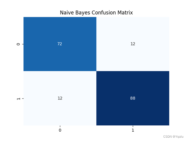
nb=GaussianNB() nb.fit(Xtrain,Ytrain) Ypred = nb.predict(Xtest) cm=confusion_matrix(Ytest, Ypred) nb_train_acc=round(accuracy_score(Ytrain,nb.predict(Xtrain))*100,2) nb_test_acc=round(accuracy_score(Ytest,Ypred)*100,2) print('Accuracy (Naive Bayes)=',nb_test_acc,'%') print('The Mean Absolute Error (Naive Bayes)=',round(mean_absolute_error(Ytest,Ypred),2)) print('Classification Report (Naive Bayes)=\n',classification_report(Ytest,Ypred)) sns.heatmap(cm,annot=True,fmt='d',cmap='Blues',cbar=False,) plt.title('Naive Bayes Confusion Matrix') plt.show()Output:
Accuracy (Naive Bayes)= 86.96 %
The Mean Absolute Error (Naive Bayes)= 0.13
4.8 Random Forest
Random Forest is a machine learning algorithm that belongs to the family of ensemble methods. It is a powerful tool for both regression and classification tasks, and is widely used in various domains.
Random Forest works by building multiple decision trees on random subsets of the training data. Each tree is trained using a different random subset of features, which helps to reduce the correlation between the trees and improve the overall performance. The final prediction of Random Forest is obtained by averaging the predictions of all the individual trees.
rdm_frst=RandomForestClassifier(n_estimators=100) rdm_frst.fit(Xtrain,Ytrain) Ypred=rdm_frst.predict(Xtest) cm=confusion_matrix(Ytest, Ypred) rdm_train_acc=round(accuracy_score(Ytrain,rdm_frst.predict(Xtrain))*100,2) rdm_test_acc=round(accuracy_score(Ytest,Ypred)*100,2) print('Accuracy (Random Forest)=',rdm_test_acc,'%') print('The Mean Absolute Error (Random Forest)=',round(mean_absolute_error(Ytest,Ypred),2)) print('Classification Report (Random Forest)=\n',classification_report(Ytest,Ypred)) sns.heatmap(cm,annot=True,fmt='d',cmap='Blues',cbar=False,) plt.title('Random Forest Confusion Matrix') plt.show()Output:
Accuracy (Random Forest)= 87.5 %
The Mean Absolute Error (Random Forest)= 0.12

4.9 Comparing Models
models = pd.DataFrame({ 'Model':[ 'Logistic Regression','K Nearest Neighbors','Linear Support Vector Machines', 'Kernel Support Vector Machines', 'Gaussian Naive Bayes','Decision Tree', 'Random Forest' ], 'Training Accuracy':[ lr_train_acc,knn_train_acc,svm_train_acc,svm_k_train_acc,nb_train_acc,tree_train_acc,rdm_train_acc ], 'Model Accuracy Score':[ lr_test_acc,knn_test_acc,svm_test_acc,svm_k_test_acc,nb_test_acc,tree_test_acc,rdm_test_acc ] }) print(models.sort_values(by='Training Accuracy',ascending=False))Output:
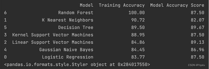
According to the result, Decision Tree model’s prediction result is pretty well. Its “Training Accuracy” is slightly lower than K-Nearest Neighbors model, and also roughly on par with the Kernel Support Vector model, but significantly higher than Linear Support Vector model, Gaussian Naïve Bayes model as well as Logistic Regression model.
Chapter 05 Conclusion
5.1 Result Interpretation
This study provides an important reference for medical diagnosis in related fields. The Decision Tree model built in Chapter 4 can help doctors and nurses to preliminarily judge whether patients have the possibility of heart disease through various indicators, and take the next line of action accordingly.
Unfortunately, due to my personal lack of relevant knowledge in the medical field, I could not give a more in-depth explanation of this model. If knowledge related to the diagnosis of heart disease is equipped, I will be able to give a deeper understanding of the meaning behind each indicator, which makes this study more focused. Moreover, I can also provide more evaluation perspectives for the effectiveness of the model, making this study more practical significance.
5.2 Modeling Process
In the modeling process, this study mainly focuses on the Decision Tree model, supplemented by other models such as Random Forest model, and K-Nearest Neighbors, etc.
However, my understanding in the field of machine learning is not enough and could not make more precise and effective adjustment or optimization of all the models. Some models are only in the primary stage thus lacking inference significance, which also makes the model comparison less contributing to the overall report. To draw a more comprehensive and in-depth conclusion, this report should first perfect each model and then compare more indicators of the prediction.
5.3 Application of Visual Tools
Visualization is key. It makes the data talkative. Displaying the present information and results of any tests or output through visualization becomes crucial as it makes the understanding easy. In other hand, we should not rely too much on charts, and a certain amount of in-depth elaboration is also necessary. From my perspective, this report is slightly out of balance in terms of graphic ratio. Too many charts and graphs make the report redundant while distracting readers from the main point.
