
阅读量:0
文章目录
目标
在本实验中,你将:使用梯度下降自动化优化w和b的过程
工具
在本实验中,我们将使用:
- NumPy,一个流行的科学计算库
- Matplotlib,一个用于绘制数据的流行库在本地目录的
- lab_utils.py文件中绘制例程
import math, copy import numpy as np import matplotlib.pyplot as plt plt.style.use('./deeplearning.mplstyle') from lab_utils_uni import plt_house_x, plt_contour_wgrad, plt_divergence, plt_gradients 当前jupyter note工作目录需要包含:
问题陈述
让我们使用和之前一样的两个数据点——一个1000平方英尺的房子卖了30万美元,一个2000平方英尺的房子卖了50万美元。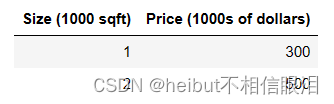
# Load our data set x_train = np.array([1.0, 2.0]) #features y_train = np.array([300.0, 500.0]) #target value 计算损失
这是上一个实验室开发的。我们这里还会用到它
#Function to calculate the cost def compute_cost(x, y, w, b): m = x.shape[0] cost = 0 for i in range(m): f_wb = w * x[i] + b cost = cost + (f_wb - y[i])**2 total_cost = 1 / (2 * m) * cost return total_cost 梯度下降总结
线性模型:f(x)=wx+b
损失函数:J(w,b)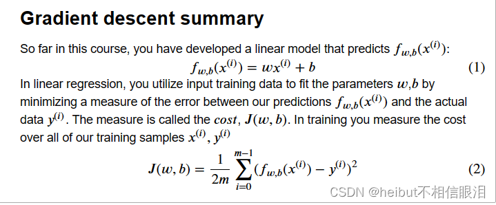
参数更新: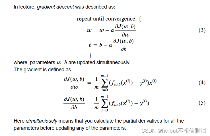
执行梯度下降
def compute_gradient(x, y, w, b): """ Computes the gradient for linear regression Args: x (ndarray (m,)): Data, m examples y (ndarray (m,)): target values w,b (scalar) : model parameters Returns dj_dw (scalar): The gradient of the cost w.r.t. the parameters w dj_db (scalar): The gradient of the cost w.r.t. the parameter b """ # Number of training examples m = x.shape[0] dj_dw = 0 dj_db = 0 for i in range(m): f_wb = w * x[i] + b dj_dw_i = (f_wb - y[i]) * x[i] dj_db_i = f_wb - y[i] dj_db += dj_db_i dj_dw += dj_dw_i dj_dw = dj_dw / m dj_db = dj_db / m return dj_dw, dj_db plt_gradients(x_train,y_train, compute_cost, compute_gradient) plt.show() 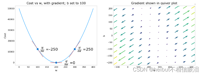
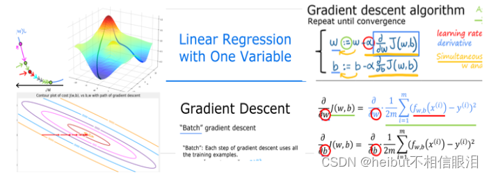
上面的左边的图固定了b=100。左图显示了成本曲线在三个点上相对于w的斜率。在图的右边,导数是正的,而在左边,导数是负的。由于“碗形”,导数将始终导致梯度下降到梯度为零的底部。
梯度下降将利用损失函数对w和对b求偏导来更新参数。右侧的“颤抖图”提供了一种查看两个参数梯度的方法。箭头大小反映了该点的梯度大小。箭头的方向和斜率反映了的比例在这一点上。注意,梯度点远离最小值。从w或b的当前值中减去缩放后的梯度。这将使参数朝着降低成本的方向移动。
梯度下降法
既然可以计算梯度,那么上面式(3)中描述的梯度下降可以在下面的gradient_descent中实现。在评论中描述了实现的细节。下面,你将利用这个函数在训练数据上找到w和b的最优值。
def gradient_descent(x, y, w_in, b_in, alpha, num_iters, cost_function, gradient_function): """ Performs gradient descent to fit w,b. Updates w,b by taking num_iters gradient steps with learning rate alpha Args: x (ndarray (m,)) : Data, m examples y (ndarray (m,)) : target values w_in,b_in (scalar): initial values of model parameters alpha (float): Learning rate num_iters (int): number of iterations to run gradient descent cost_function: function to call to produce cost gradient_function: function to call to produce gradient Returns: w (scalar): Updated value of parameter after running gradient descent b (scalar): Updated value of parameter after running gradient descent J_history (List): History of cost values p_history (list): History of parameters [w,b] """ w = copy.deepcopy(w_in) # avoid modifying global w_in # An array to store cost J and w's at each iteration primarily for graphing later J_history = [] p_history = [] b = b_in w = w_in for i in range(num_iters): # Calculate the gradient and update the parameters using gradient_function dj_dw, dj_db = gradient_function(x, y, w , b) # Update Parameters using equation (3) above b = b - alpha * dj_db w = w - alpha * dj_dw # Save cost J at each iteration if i<100000: # prevent resource exhaustion J_history.append( cost_function(x, y, w , b)) p_history.append([w,b]) # Print cost every at intervals 10 times or as many iterations if < 10 if i% math.ceil(num_iters/10) == 0: print(f"Iteration {i:4}: Cost {J_history[-1]:0.2e} ", f"dj_dw: {dj_dw: 0.3e}, dj_db: {dj_db: 0.3e} ", f"w: {w: 0.3e}, b:{b: 0.5e}") return w, b, J_history, p_history #return w and J,w history for graphing # initialize parameters w_init = 0 b_init = 0 # some gradient descent settings iterations = 10000 tmp_alpha = 1.0e-2 # run gradient descent w_final, b_final, J_hist, p_hist = gradient_descent(x_train ,y_train, w_init, b_init, tmp_alpha, iterations, compute_cost, compute_gradient) print(f"(w,b) found by gradient descent: ({w_final:8.4f},{b_final:8.4f})") 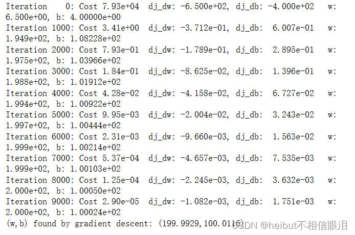
成本与梯度下降的迭代
代价与迭代的关系图是衡量梯度下降过程的有用方法。在成功的运行中,成本应该总是降低的。最初成本的变化是如此之快,用不同的尺度来绘制最初的坡度和最终的下降是很有用的。在下面的图表中,请注意轴上的成本比例和迭代步骤。
# plot cost versus iteration fig, (ax1, ax2) = plt.subplots(1, 2, constrained_layout=True, figsize=(12,4)) ax1.plot(J_hist[:100]) ax2.plot(1000 + np.arange(len(J_hist[1000:])), J_hist[1000:]) ax1.set_title("Cost vs. iteration(start)"); ax2.set_title("Cost vs. iteration (end)") ax1.set_ylabel('Cost') ; ax2.set_ylabel('Cost') ax1.set_xlabel('iteration step') ; ax2.set_xlabel('iteration step') plt.show() 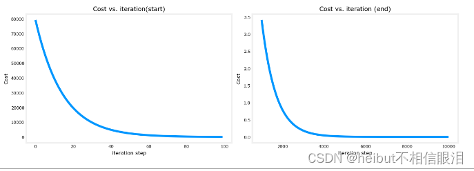
预测
现在您已经发现了参数w和b的最优值,您可以现在用这个模型根据我们学到的参数来预测房价。作为预期,预测值与训练值几乎相同住房。此外,不在预测中的值与期望值一致。
print(f"1000 sqft house prediction {w_final*1.0 + b_final:0.1f} Thousand dollars") print(f"1200 sqft house prediction {w_final*1.2 + b_final:0.1f} Thousand dollars") print(f"2000 sqft house prediction {w_final*2.0 + b_final:0.1f} Thousand dollars") 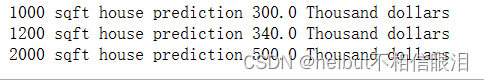
绘制
您可以通过在代价(w,b)的等高线图上绘制迭代代价来显示梯度下降的执行过程。
fig, ax = plt.subplots(1,1, figsize=(12, 6)) plt_contour_wgrad(x_train, y_train, p_hist, ax) 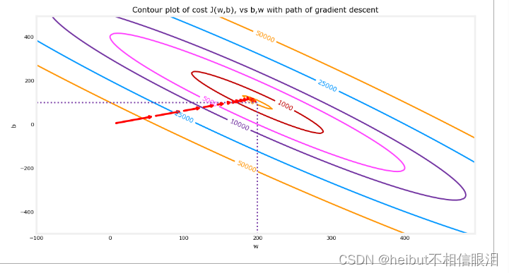
上图等高线图显示了w和b范围内的成本(w, b)用圆环表示。用红色箭头覆盖的是梯度下降的路径。以下是一些需要注意的事项:这条路平稳地(单调地)向目标前进。最初的步骤比接近目标的步骤要大得多。
放大后,我们可以看到梯度下降的最后步骤。注意,当梯度趋于零时,步骤之间的距离会缩小。
fig, ax = plt.subplots(1,1, figsize=(12, 4)) plt_contour_wgrad(x_train, y_train, p_hist, ax, w_range=[180, 220, 0.5], b_range=[80, 120, 0.5], contours=[1,5,10,20],resolution=0.5) 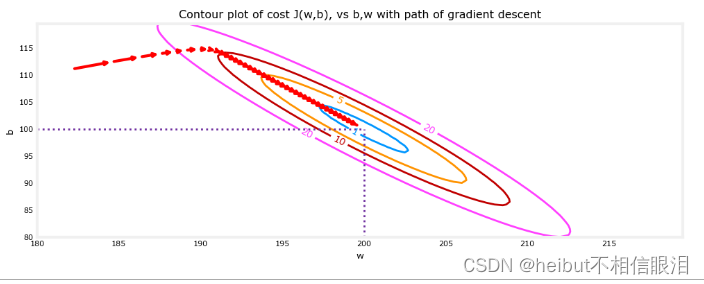
# initialize parameters w_init = 0 b_init = 0 # set alpha to a large value iterations = 10 tmp_alpha = 8.0e-1 # run gradient descent w_final, b_final, J_hist, p_hist = gradient_descent(x_train ,y_train, w_init, b_init, tmp_alpha, iterations, compute_cost, compute_gradient) 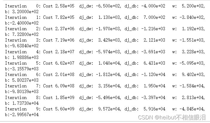
上面,w和b在正负之间来回跳跃,绝对值随着每次迭代而增加。此外,每次迭代J(w,b)都会改变符号,成本也在增加W而不是递减。这是一个明显的迹象,表明学习率太大,解决方案是发散的。我们用一个图来形象化。
plt_divergence(p_hist, J_hist,x_train, y_train) plt.show() 上面,左图显示了w在梯度下降的前几个步骤中的进展。W从正到负振荡,成本迅速增长。梯度下降同时在两个魔杖b上运行,因此需要右边的3-D图来获得完整的图像。
祝贺
在这个实验中深入研究了单个变量的梯度下降的细节。开发了一个程序来计算梯度想象一下梯度是什么完成一个梯度下降程序利用梯度下降法求参数考察了确定学习率大小的影响
