The basics of neural signal processing
course from youtube: 传送地址
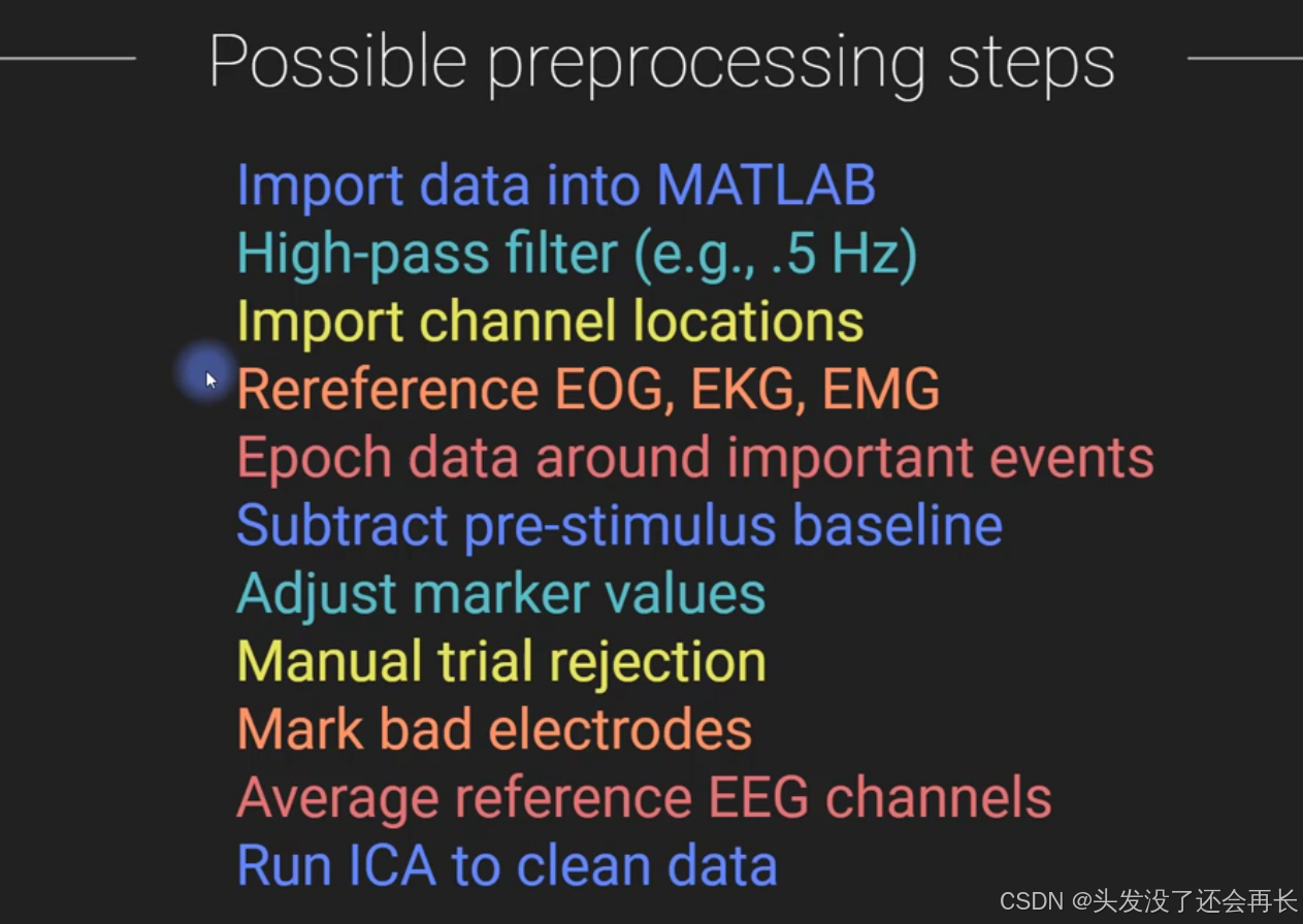
Possible preprocessing steps
Signal artifacts (not) to worry about
doing visual based artifact rejection so that means that before you start analyzing, you can identify those data epics and simply remove them or make a decision about whether you think that it might be possible to isolate and separate out that artifact.
here you see these 64 channels EEG data.
In the middle, there are some big deflections appear in many channels, so these turn out to be this is each time the subject blinked their eye.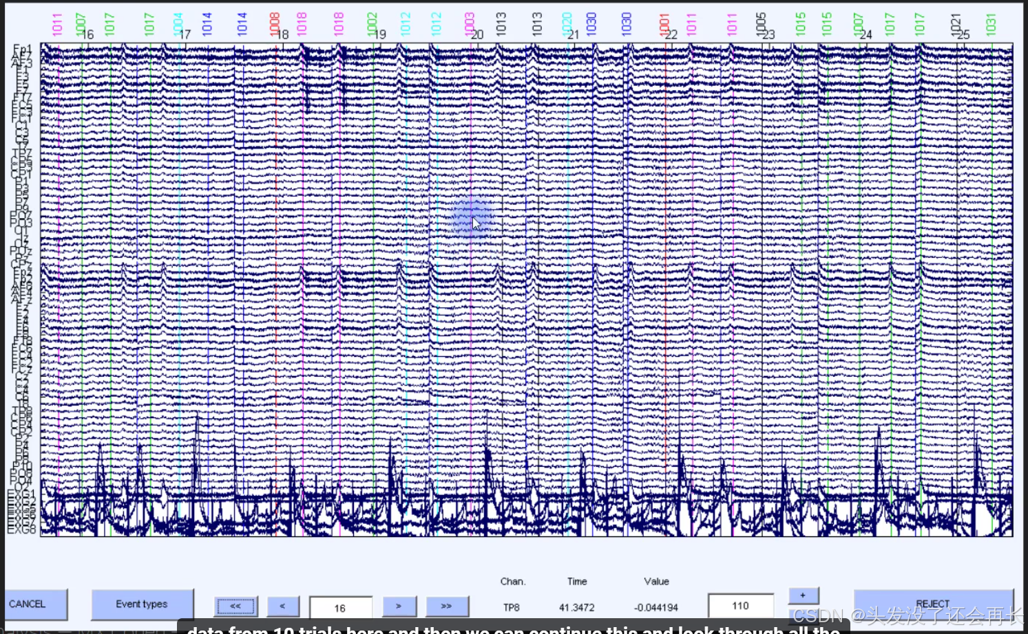
Topographical mapping
this shows a layout withe 64 electrodes, the electrodes are positioned on the scalp and you can see that there are colors all everywhere.
we actually didn’t measure any data at this point there was no data measured except for exactly where these black dots. and so how can we draw the colors here if we didn’t actually measure any data well this is done based on something called interpolation.
what was happening at this time point in the experiment(the left topographical map) , the answer is that at this time point in the experiment there was a visual stimulus that was shown on a computer screen so here you can see activity in posterior regions corresponding to the activation of visual cortex.
that’s
what we see here here the subject made a response they pressed a button with the right hand (the right topographical map) and we see activation of this kind of central lateral sensory motor area here.
so we can already determine a lot about what’s happening in the experiment just based on looking at the topographical maps.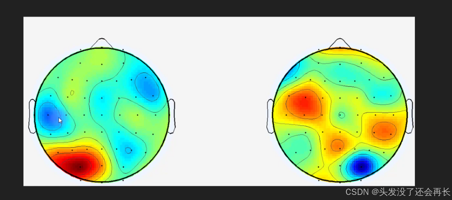
here you see another advantage of looking at topographical maps and that is to identify potentially bad electrodes so what I’ve done here this is actually a clean dataset this is showing the top of ethical maps at different time points of the number in this box corresponds to time points in milliseconds after a stimulus onset so that’s already interesting you can see how activity is unfolding over time and what I’ve done here in this otherwise clean dataset is replace one electrode with pure noise.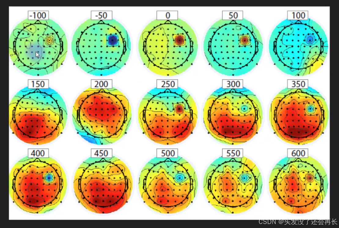
Electrode labeling conventions
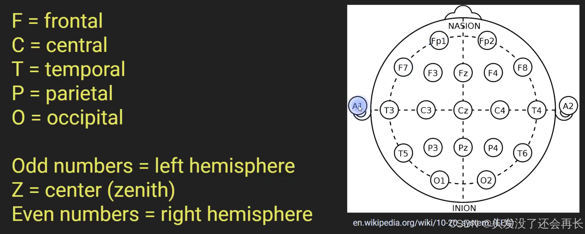
every electrode gets first a letter or sometimes two letters and then it gets a number so we have a combination of letters and numbers and the letters indicate the topographical region.
sometimes you get these extra letters so in this case this would be frontal pole you can see here is the the frontal pole so this is even more anterior than the F channel so that’s called FP.
the odd numbers are in the left hemisphere.
the even numbers are in the right hemisphere.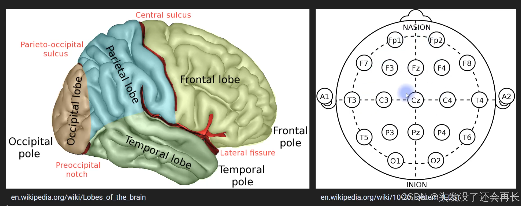
overview of time-domain analyses(ERPs)
what do you notice about the relationship between the event related potential and the single trial voltage fluctuations which you’ve probably noticed is that it’s quite a bit smaller it’s around an order of magnitude
smaller the ERP tends to be around an order of magnitude smaller than the single trial variability.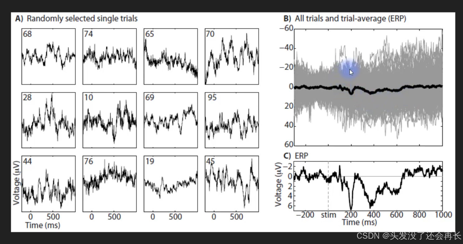
this called phase-locked or non-phased signals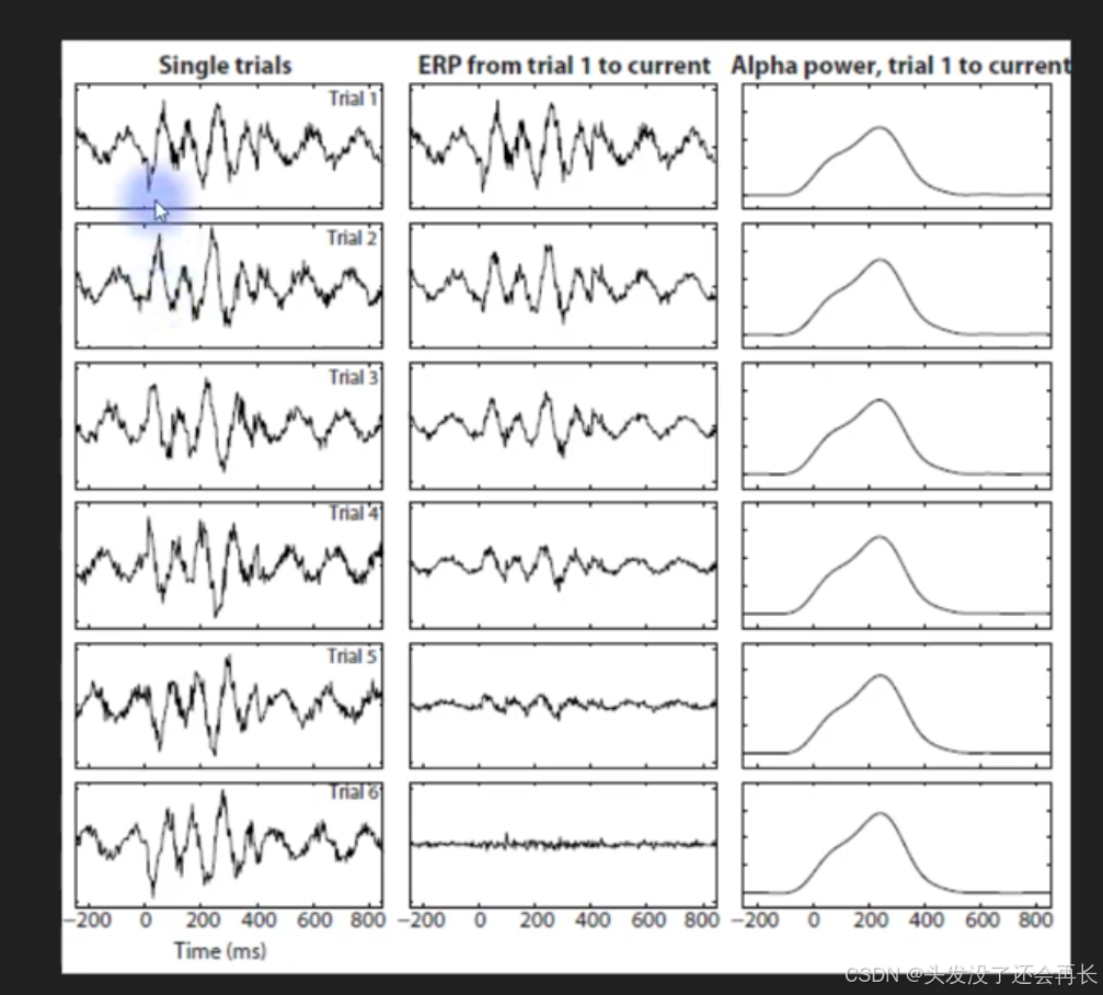
Motications for rhythm-based analyses
b is the time frequency from trail 1 to 3, and then the right here you see that these narrowband frequency rhythms here are present in the time frequency plot here and then what you see here is the average of these there individual over all of those three individual plots. then you see both the phase-locked response and the non phase-locked response in the same signal so by applying these time frequency analysis we are extracting **more information from the signal ** than what we get from just from ERP.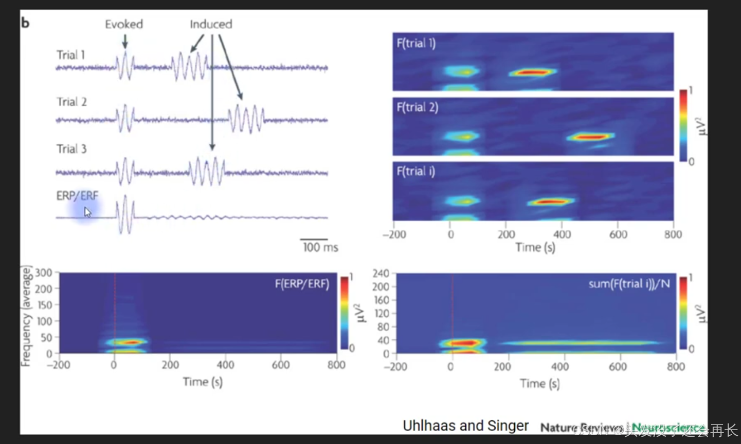
when something is phase-locked and time locked then you will see it in the time frequency analysis and you’ll see it in the event related potential.
if something is time locked if the activity is time locked but non phase locked then you get this situation that the event related potential goes to zero.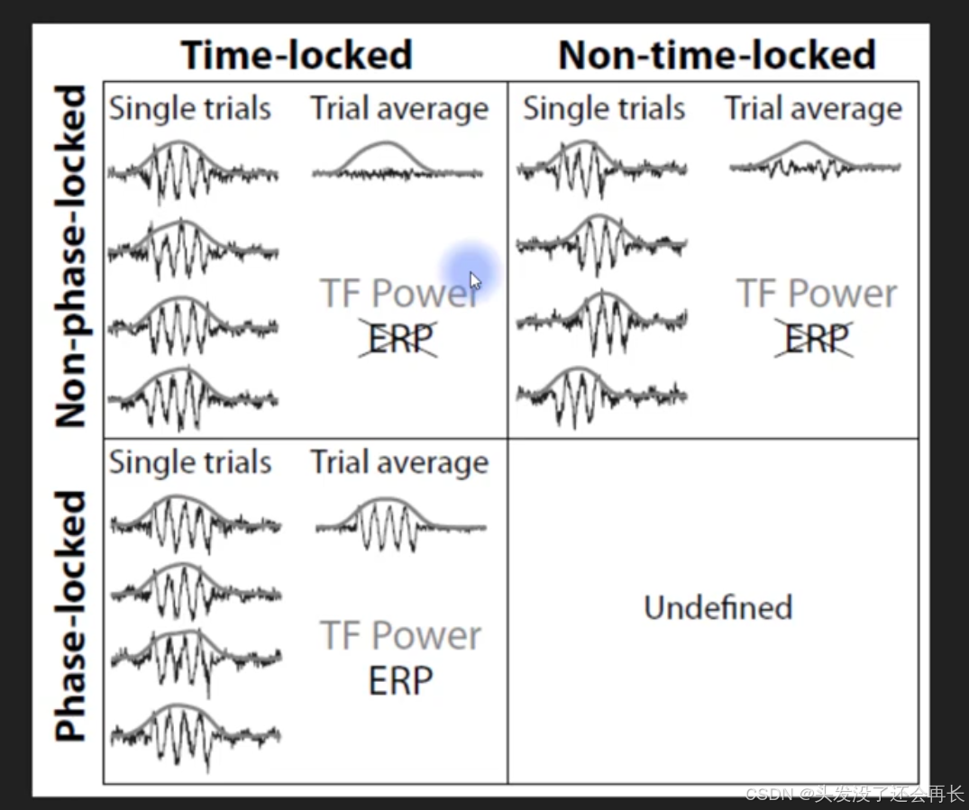
Studying the brain in the lab
Two methods : Imaging and Electrophysiolog
Interpreting time-frequency plots
the left is a signal in the time domain. and the right we have a graph that’s going to be in the frequency domain this is going to be a power spectrum that we are going to build.
build a power spectrum from this time domain signal that’s done through an operation called the Fourier transform.
the general idea of how the Fourier transform works is that you start with your signal and then you take a sine wave this is a pure sine wave at some frequency and you just line them up on top of each other and then you ask the question how similar does this signal look like the sine wave.
then you calculate how similar is the signal and the sine wave and generate a plot so a bar at this particular frequency corresponding to the frequency of the sine wave.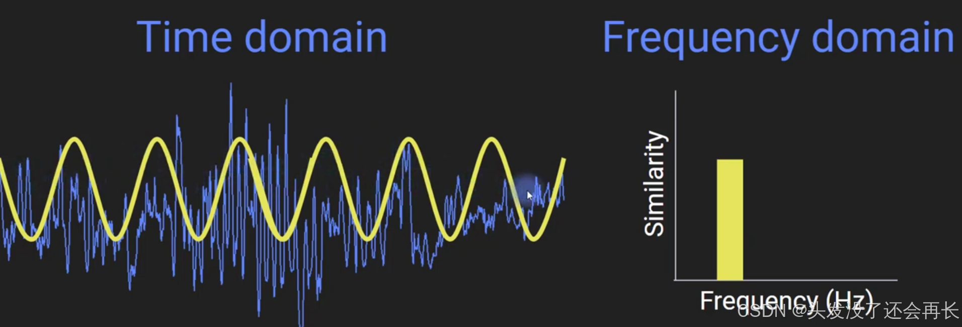
end of this signal and when you repeat this procedure for many different frequencies so different sine waves with different frequencies you are going to end up building up a spectrum that looks like this so here you see the frequency of the sine wave .
this y-axis here corresponds to like the amount of similarity or the energy between the signal and the sine wave at these different frequencies now this particular graph is shown in a relative.
but those temporal dynamics are not visible in the spectrum and that’s why I call this a static spectrum.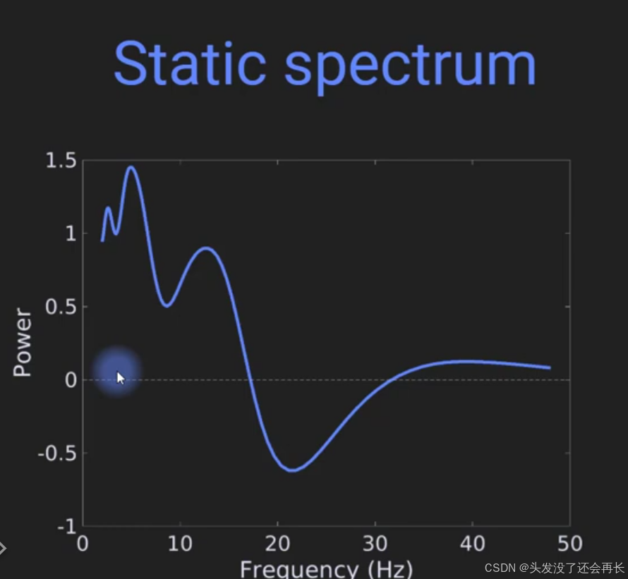
so what we want to do is basically take this representation and split it up over different parts of the time window.
this is
called well here I call it a dynamic spectrum but it’s called a time frequency plot and it’s called a time frequency plot because it shows how information changes over time.
the static spectrum plot just from one time window, so you can imagine that you would color these positive values red and these negative values blue and then you could like spin this or rotate this line so that it’s one column in this matrix so here you can see at lower frequencies it’s red that means its positive here and at higher frequencies it gets blue its negative.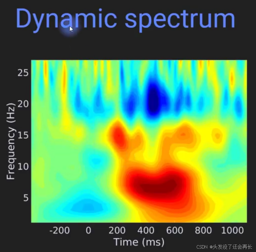
How to inspect time-frequency results like a pro
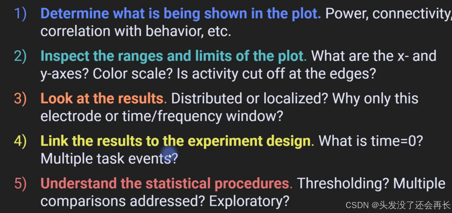
this is an example: five step plan
step one: we can see the title is db-convert TF power plot, so it’s a db convert time frequency power graph
step two: we see that it is a symmetric color scale, the negative side and the positive side are the same magnitude and that also tell us that zero which is relative so no relative changes in power correspinds to this green color. the time axes go from looks like minus 300 milliseconds up to one second so in total we have around a second and a quarter or a second and a third of time. the frequency axes we can see the lowest frequency maybe one or two hertz and it goes up to hertz.
step three: distributed or localized? you see this blue patch is kind of fairly distributed over time it seems to last for 800 or maybe 900 milliseconds so it’s almost a second but it’s fairly limited in frequency so it’s most of this goes from 20 to 25 hertz and this little burst that goes up to 390 hertz. and we can also see a couple of other features(red) here that all tend to be a little bit band-limited so they are existing in a narrow frequency band so narrow on the y axis is relevant for interpreting time frequency features because to interpret something as an oscillation as a narrowband activity. whether there are features in a time frequency plot that cut off by the axes. (consider about axes)
step four: link the results to the experiment design.
step five: but we can’t determine whether the results is meaningful or not.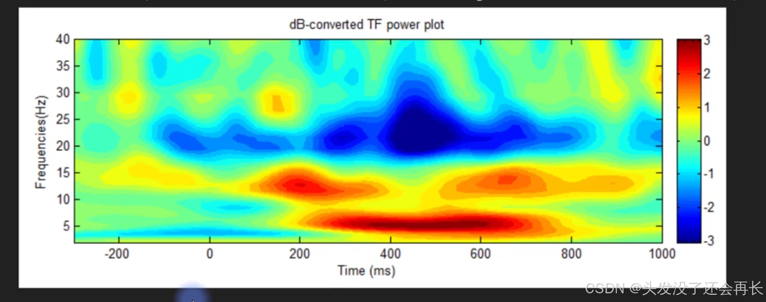
Where to get more EEG data?

Simulating noise for analysis evaluation
to crate white noise we can draw numbers from two different distributions a normal distribution of course is also a Gaussian distribution or a bell-curve distribution where the probability is highest for numbers that are close to zero. and we have a uniform distribution of noise where all the values between 0 & 1 are equally likely to be selected and there’s no possibility of getting number less than 0 or greater than 1.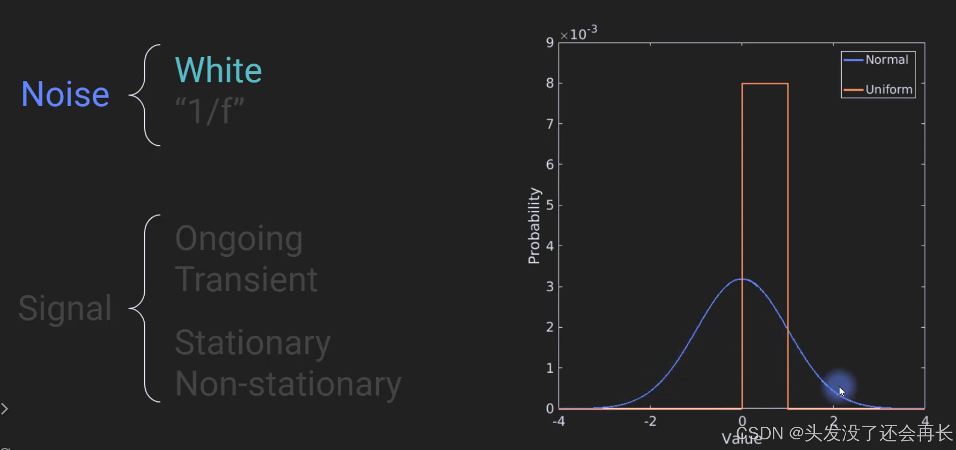
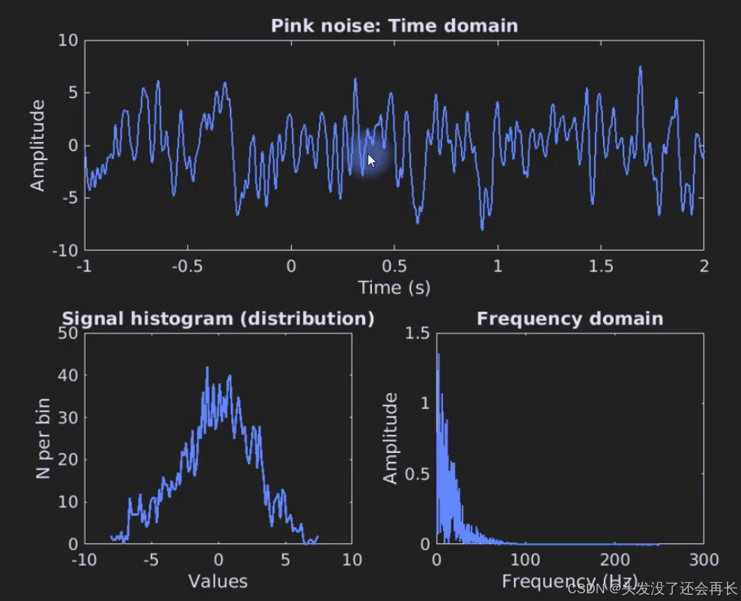
we actually focus on ongoing signals one of that is through a sine wave and the we can else change this formula around a little bite or add some modification to this basic sine formula to generate more interesting and non stationary patterns.
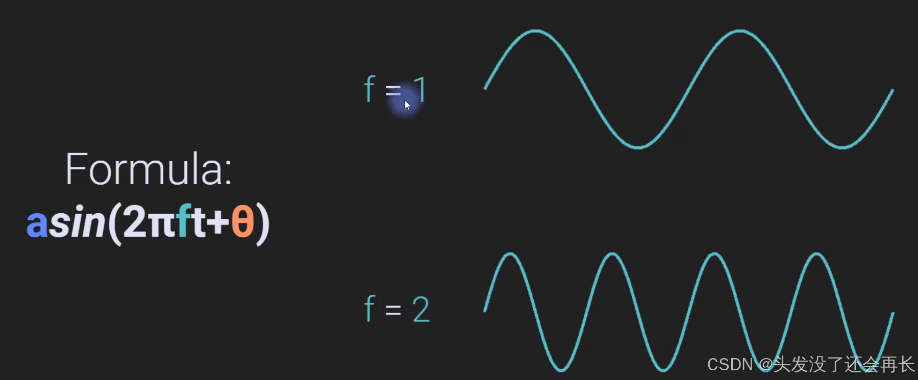
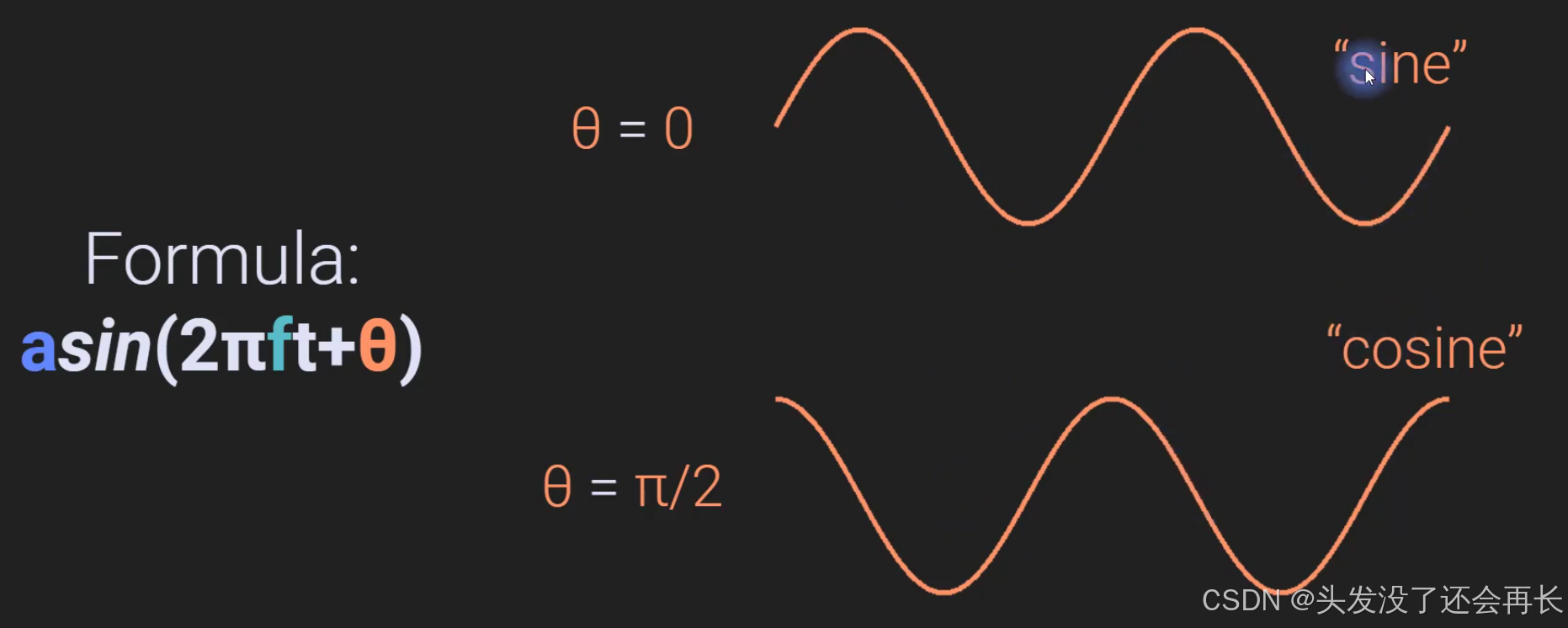
the formula for the sine wave, a is an amplitude parameter so it defines basically the height of this curve. f is frequency which defines the speed of the oscillation. t is time typically in seconds and theta is a parameter that defines the speed shift on the x axis so kind of taking this whole function and sliding it back and forth so left and right on the x axis.
it’s a stationary signal because its properties are not changing over time so it has one parameter for amplitude and that is constant over time .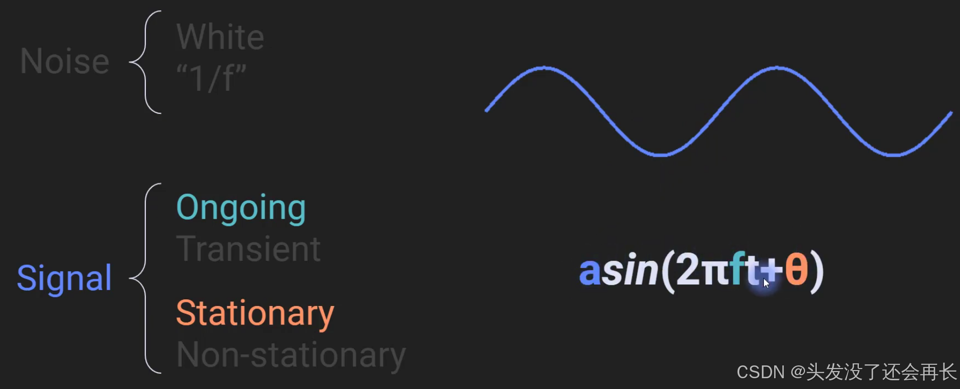
we can modify this to have a non stationary ongoing signal, just like the below graph, the frequency is changing over time, the sine wave is faster and then slower and then faster…
the xt formulate that governs this time series and so what you do is you start with a vector f that is the istaneous frequency that you want, the delta is data sampling rate, t is the time, k would be the individual time point and this generates some other vector called X and then X goes into sine function. it’s sine 2pi times the quantity xt plus tt. tt is the TF time point in the vector of time points and that generates each each time point in the output vector y.
why we create data in a way that looks like this is that this is actually a closer approximation to the kinds of signals that actually measured in real brain signals.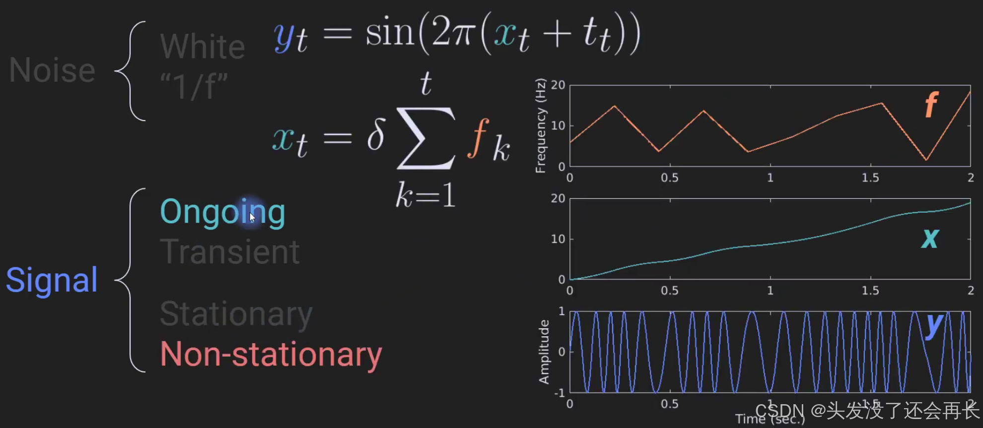
here we are primarily going to talk a little bit about generating transient activity.
This is a Time domain Gaussian equation y, a=1.5 c=0.5 h=1.1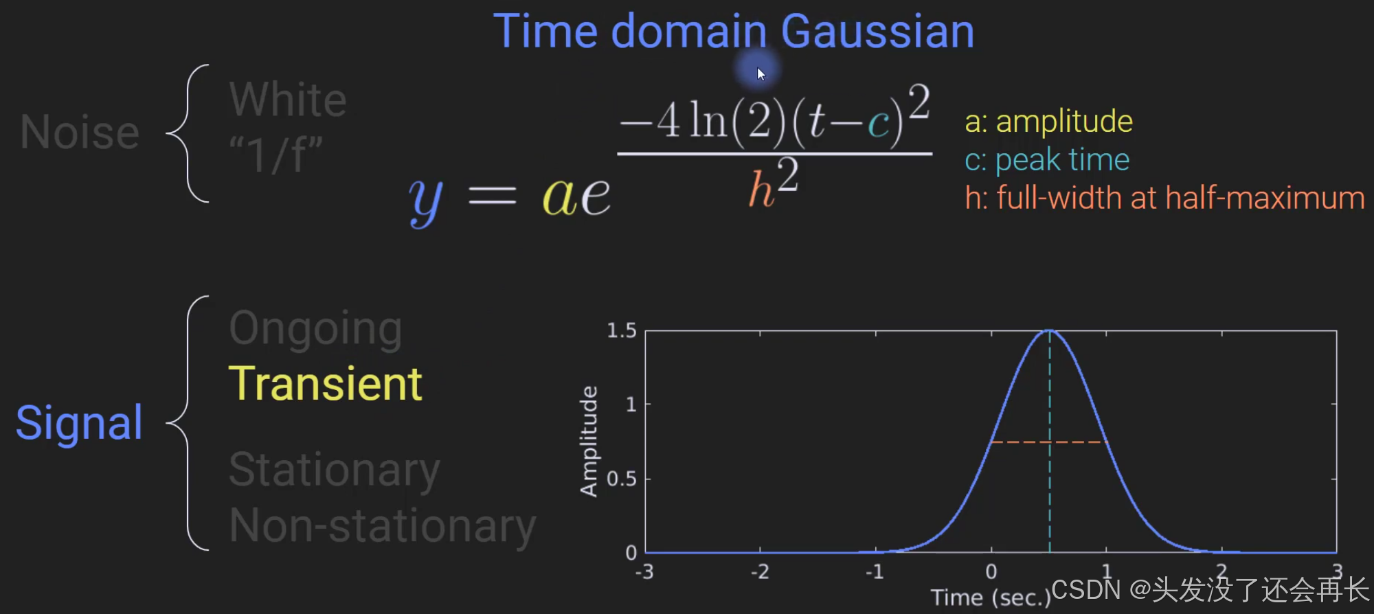
This is a frequency domain gaussian. the idea of creating a guassian frequency domain is take the inverse Fourier transform of this shape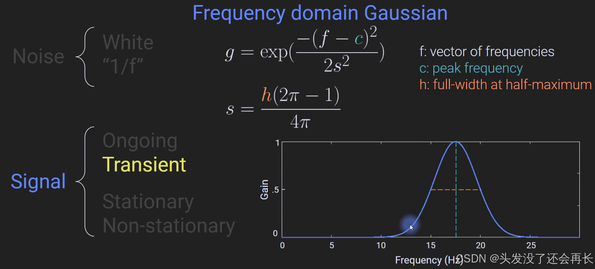
Time and frequency domains
the way from time domain to frequency domain is count the number of rhythms the number of pulses or repetitions cycles that we see in the period of one second , we see int the first time graph, there is three cycle, so get a bar here at 3 Hertz then the height of this bar is 1 here.
the third graph is first graph plus second graph, it has two components one at three Hertz with an amplitude of one and one at five Hertz with amplitude of two.
at five here highlights one of the frequency-domain compared to the time domain and that is that if the signal contains rhythmic narrow compañero band components which is the case here it’s not the case for all signals but if the signal is made up of narrowband spectral features then you can understand the signal much better and much faster when looking at the signal in the frequency domain compared to the time domain again.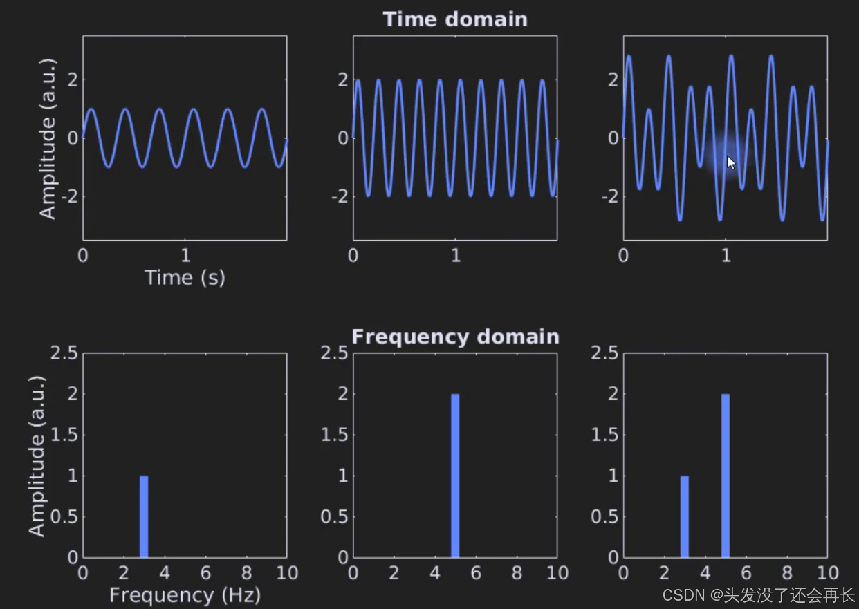
here you can count five this is gonna be much harder you’re not really going to be able to guess that this is a three Hertz sine wave plus a five-foot sine. but when you look at it in the frequency domain it is totally trivial you see immediately that we have a three Hertz sine wave component with an amplitude of 1 plus broadband noise with low amplitude and the same story here and same story here.
when you add up all of these little and contributions of small power for a lots and lots of frequencies in the time domain that ends up being a large amount of noise even though for any individual frequency it’s quite small so therefore looking at a signal in the frequency domain can also improve the signal to noise characteristics of interpreting the signal and that is the second advantage of the frequency domain.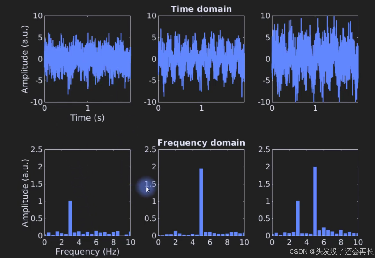
Computational foundations of the Fourier transform
simulating ongoing sine waves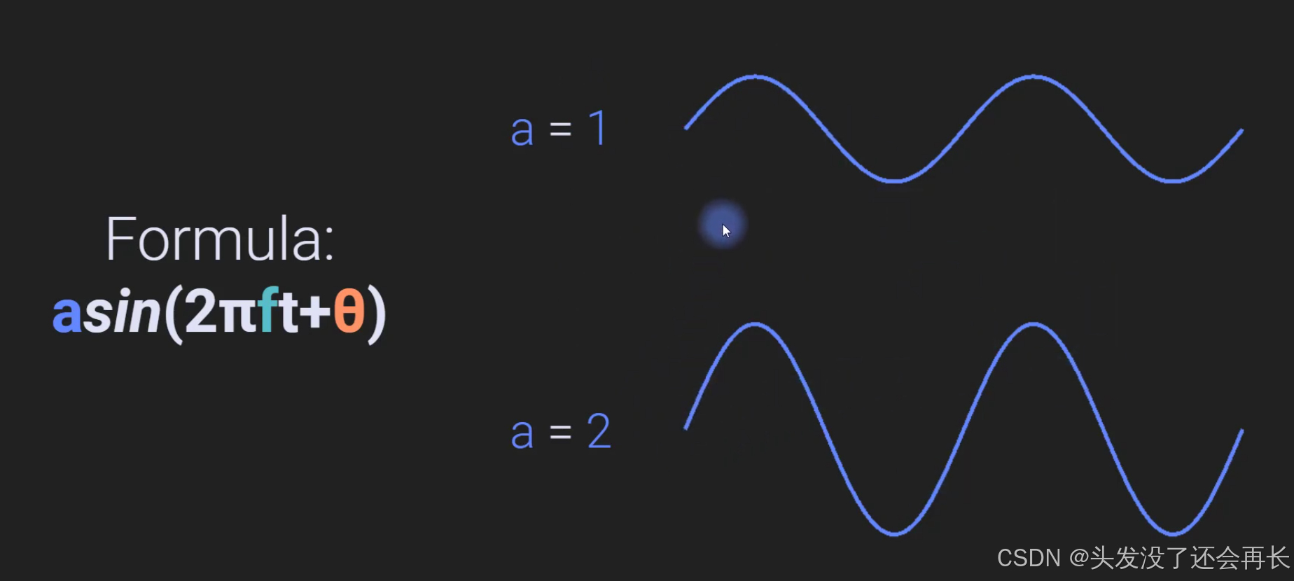
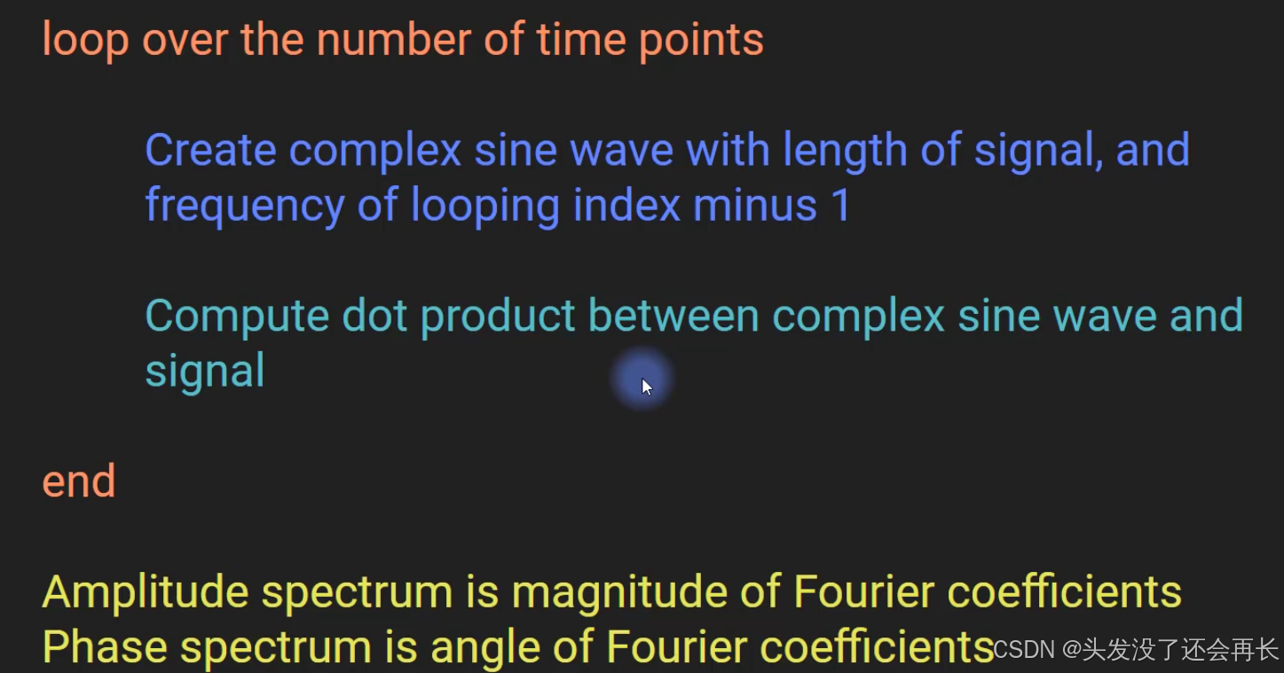
How the DTFT works(loop algorithm)
we want compute the dot product between the sine wive and the signal(dot product is valid only when both vectors in this case the signal and the sine wave have the same number of numbers). now you can imagine that the dot product between this sine wave and the signal is going to be large because they look really similar.
the magnitude of that product gets plotted on the y-axis at the x-axis location corresponding to the frequency of this sine wave.
the dot product the real value dot product between the sine wave and a signal is very much dependent on the phase of signal , the signal of the sine wave.
then we move on to some other frequency, so if we use this yellow sine wave, the dot product is not going to be as large and that is why we need to use a complex valued sine wave and not just a real valued sine wave. complex valued sine wave accounts for any possible phase relationship between the signal and the complex valued sine wave and that phase offset is handled because the signal is going to look something like the cosine.
so the procedure gets repeated for lots of sine waves.
think about a high dimensional space where each dimension each axis is defined by a signal time point, if you have a signal that has 700 time points, then is space is going to be a 700 dimensional space. each axis correspond to the millivolt or microvolt.
so the signal plot to this space is a vector, the sine wave is just some other waves, the signal is a real-valued signal and this is a real-valued space. we can compute the dot product of the signal and csw, we all the dot product “Fourier coefficient”, m is amplitude and theta is phase.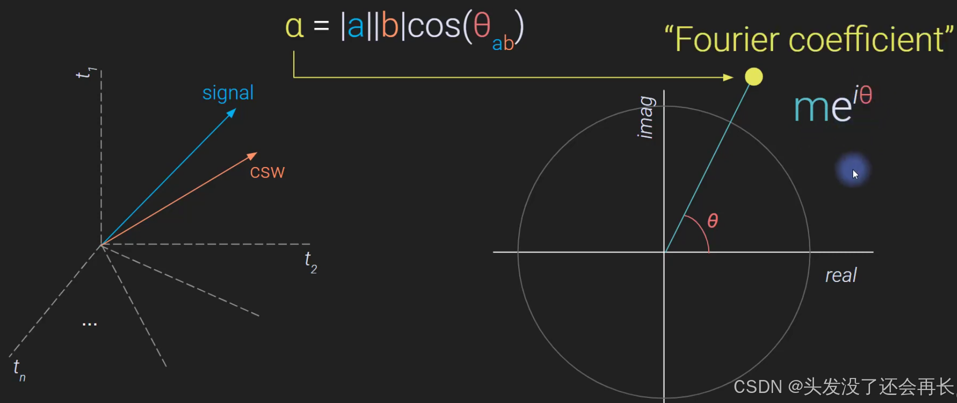
The formula to convert indices to Hz
N is the number of time points, so the time points int the signal defines the number of frequency or frequency resolution that we can extract from that signal.
first we create a complex valued sine wave, the fourierTime is a normalized time vector goes from 0 to 1 in n steps where n is the number of time points in the signal. this sine wave here the units are not in Hertz, these are frequencies in indices. (so the fouriersin is a sine wave, have the same time points with signal, and the vector of sine wave from 0-1.) this is a very important feature of the Fourier transform because you want the Fourier transform to be a general operation that always works so you don’t want to have a different Fourier transform for when you sample your data in milliseconds and a different Fourier transform if you sample your data in days.
second part to compute fourier coefficient. so if we finished this loop we have all these Fourier coefficients for each frequency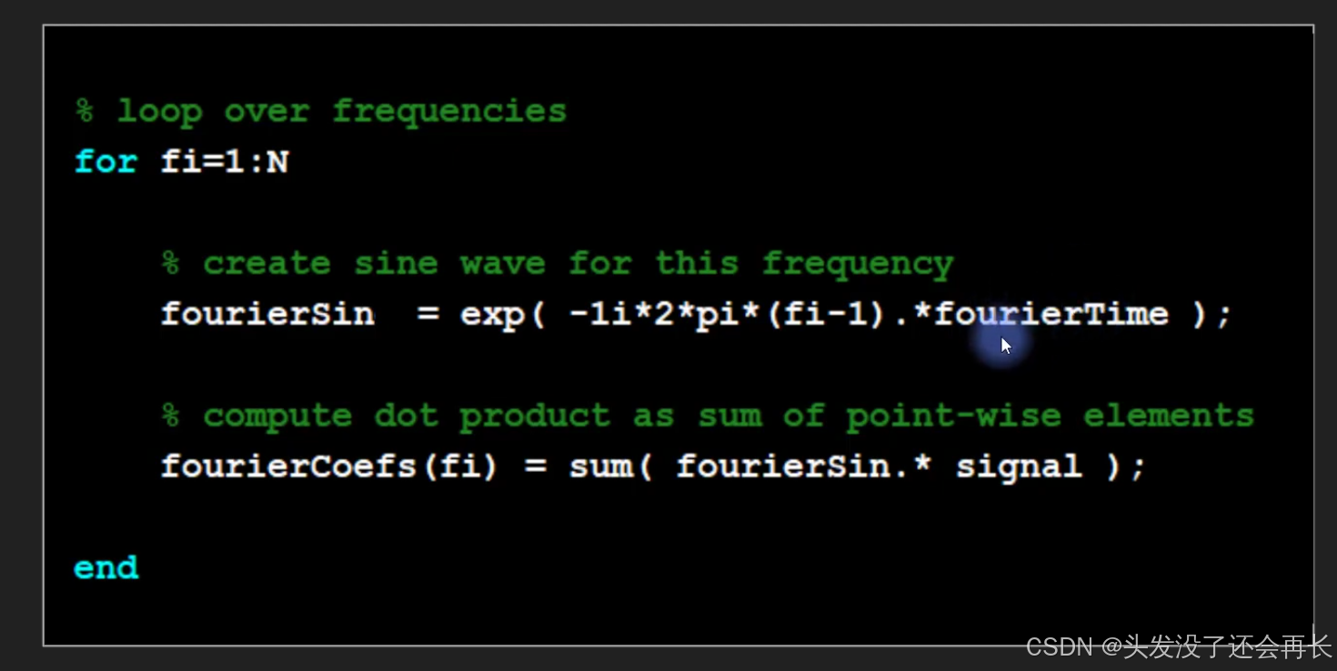
but what we want to do for spectral analysis and subsequent time frequency analysis is to interpret these Fourier coefficients in terms of their frequency in Hertz right that’s what we care about we care about physical units of Hertz.
so how do we convert from these indices these looping indices into units of Hertz well this is the formula we say that the vector of Hertz is linearly spaced numbers from zero to the sampling rate divided by two in n divided by 2 plus 1 steps so this sampling rate divided by 2 is called the Nyquist frequency. n is the time point in signal. every element in this vector represent a frequency.
Now we discuss how lower and higher bound on frequency
lower bound on frequencies
we can have a frequency of 0, that’s just a flat line, this is often called DC where DC stand s for direct current that comes from engineering. we can back to the code of the fourier transform, in the first iteration of the loop, fi equals 1, fi minus 1 is 0, then you have basically all of this turns to 0 because we’re multiplying by 0 so that gives us e to the 0 and any number to the power of 0 any number raised to 0 is 1 so this here for the first iteration of this loop this quote-unquote complex sine wave is actually just a vector of all ones and then what do we do here we are computing the dot product of the signal and a vector of all ones which really just means that we’re adding all of the signal values all the values in the signal get added up together and then later we divide by n we divide by the number of numbers and then that literally gives us the average value of the signal.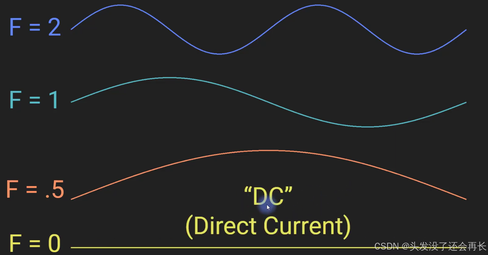
Upper bound to frequencies
theory two samples per cycle is the absolute minimum number of samples that you need to accurately reconstruct a fluctuating signal like this. so that means our upper bound is two points per cycle which means one half of the sampling rate and that is called the Nyquist frequency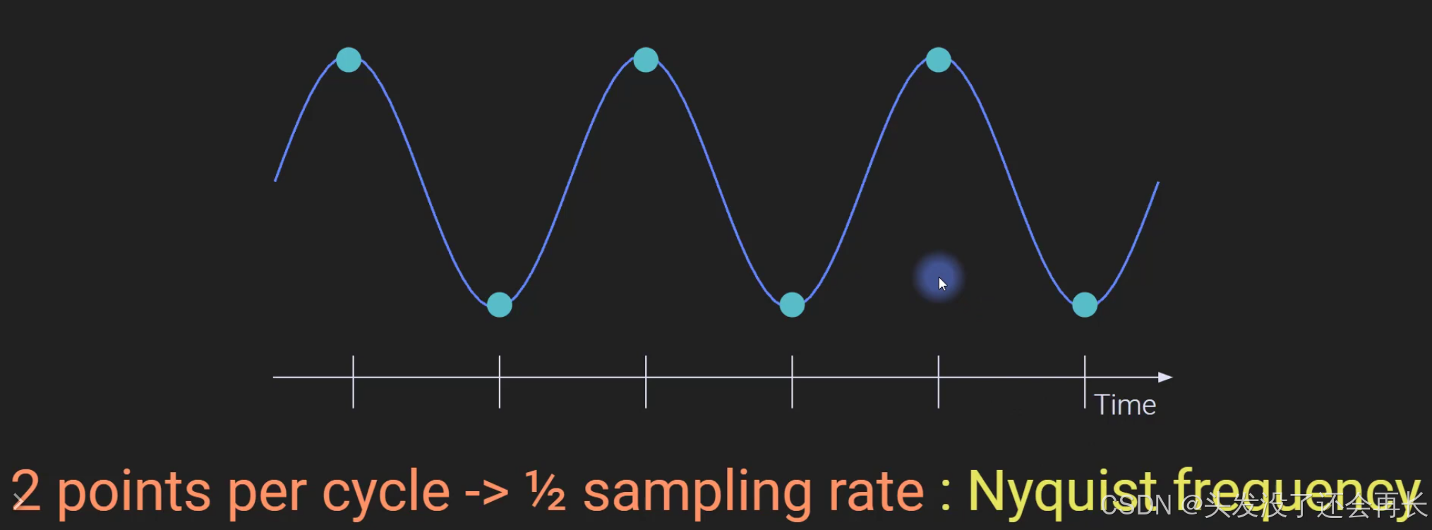
so the formula for converting frequencies from arbitrary indices into units of Hertz.
Positive and negative frequencies
to complex signal, the Fourier transform contains real-value signals and complex signals because complex signals contain phase information.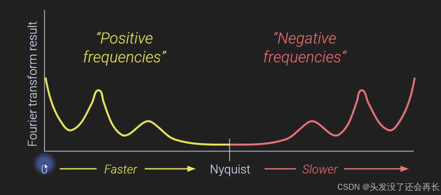
The Fourier transforms we are using complex sine waves Euler’s formula complex sine waves to represent all of the information in a real-valued signal. so how can we get a real-valued signal from complex valued numbers complex valued sine waves the answer is we have to follow this formula.
how can we get this formula? why there is a 1/2? for example: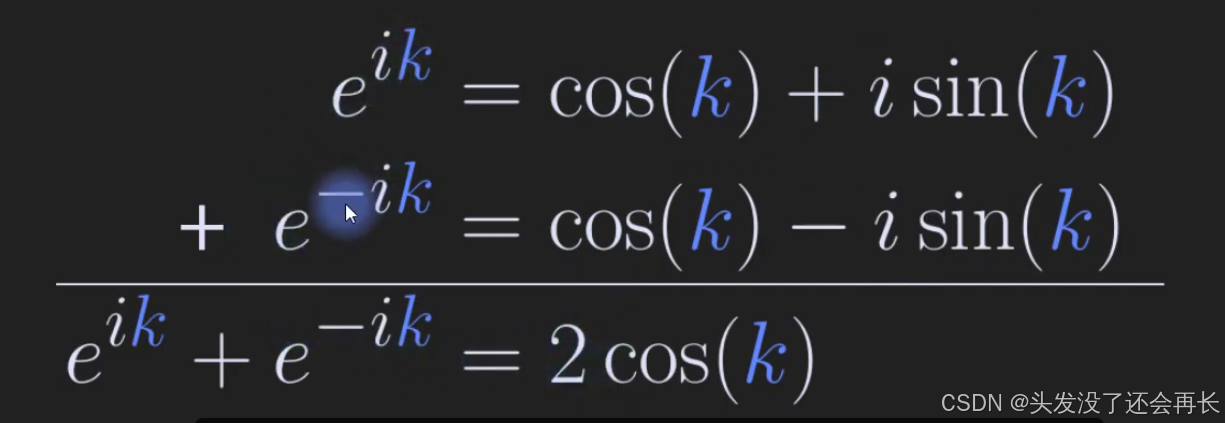
so now we can understand why the formula for converting frequencies from arbitrary indices into units of Hertz, the step is N/2+1. the for n over two plus one we have n over two because half of the spectrum is to the left of Nyquist so the positive frequencies and then the plus one because the zero Hertz we keep that on the left side of the spectrum.
why we need exactly n frequencies in the fourier transform, why we need negative frequencies is that we need to make sure that the Fourier transform is perfect invertible transform without any loss. we do not want approximate a signal we want to quantify it exactly.
but we need to know, these frequencies are going to be correct only up until the Nyquist frequency, above the Nyquist frequency is no longer be valid. so the formula is just a coding trick, if you sampling rate is 1000Hz, and 990Hz it’s actually minus 10.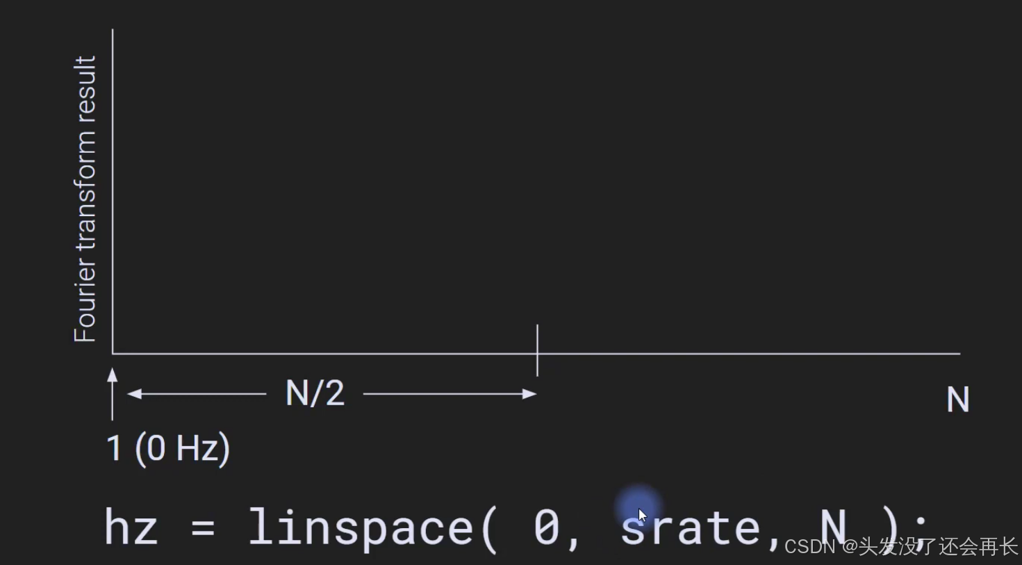
Accurate scaling of Fourier coefficients
the output of the FFT function has units that are basically uninterpretable and that will lead to a discussion of two scaling factors two normalization factors that you can apply to the Fourier coefficients in order to interpret or put the Fourier coefficients back into the units of the original data.
here is a few lines of Matlab code essentially just taking the sine of some numbers, the amplitude of this sine wave is 1, the take the FFT functions, the output of FFT function is the series of Fourier coefficients which the use abs function. the function will extract the magnitude which is the distance from the origin of each Fourier coefficient.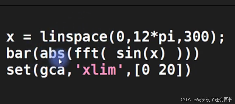
so we will get this bar, the amplitude is almost 150, because the amplitude of sin wave is 1, in the loop over frequencies, if fi = 1, the fouriersin = exp(0) = 1, so the fouriersin . * signal = signal, then the sum will to get larger and larger because we just summing together more and more numbers.
if we want to get the average value of the signal we have to divide by the number of data points in the signal that gives us the average. understand to internalize when thinking about the zero Hertz frequency so this is one of the two normalization factors for a for the Fourier coefficients.
you’re computing a lot of sums here so then we want to divide by n and that is like an average that’s basically taking the average of the relationship between the complex sine wave and the signal now let’s go back here and look at this so the number of points in this time series here is 300 so if we were to divide this by 300 that would bring this from 150 down to 0.5 it would bring us down to 1/2 and now that is still not exactly the right answer the right answer should be 1 because the amplitude of sin(x) is 1.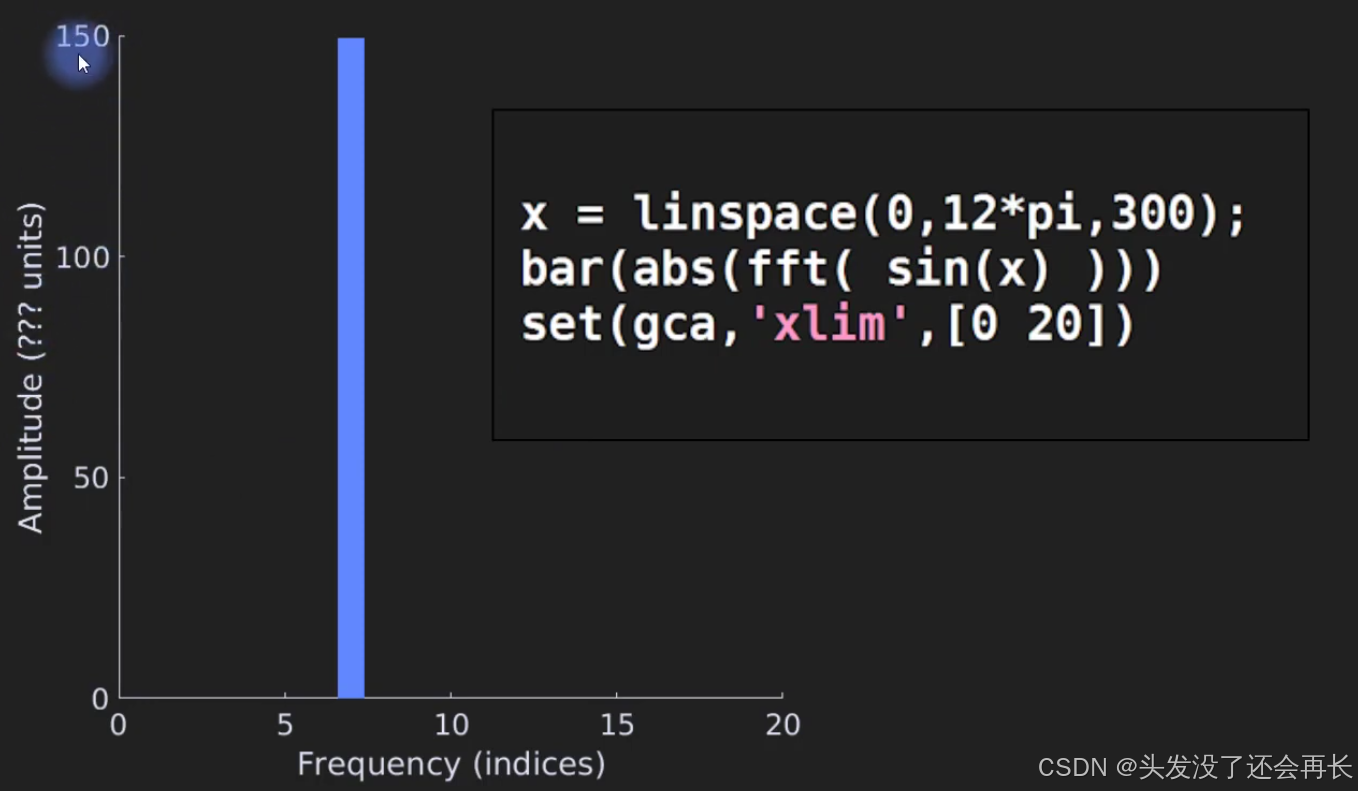
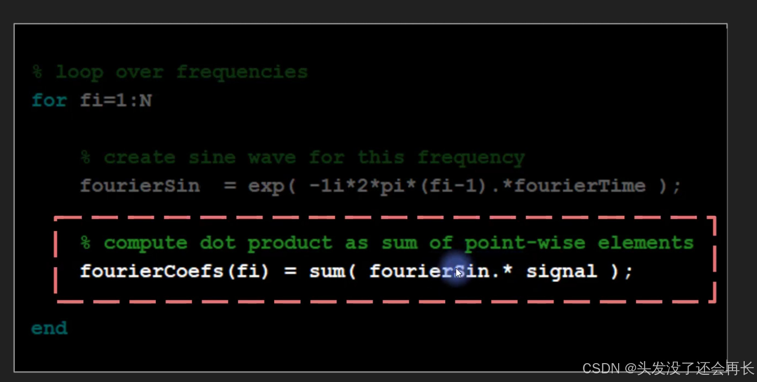
so what is the second normalization factor is to multiply by two. because the amplitude gets split between the positive frequencies and the negative frequencies so we can double the positive frequencies and then ignore the negative frequencies now just to be clear the doubling is valid.
that these two scaling factors are linear multiplicative factors they change the y-axis values but they do not change the shape of the spectrum so the spectrum is not going to look any different if you have if you apply or don’t apply these two normalization factors and therefore scaling is not always necessary scaling the so applying these two normalization factors is necessary only if you want the results of the Fourier transform to have the same units as the original signal.
zero also the Nyquist but we are particularly concerned with the zero Hertz frequency is not doubled it’s not doubled because zero has no corresponding negative frequency.
The perfection of the Fourier transform
the goal of the Fourier transform is to get a time domain signal into the frequency domain that transformation from the time domain into the frequency domain is absolutely perfect it is lossless. the Fourier transform is not an approximation of the signal it is an exact representation of the signal so no information is loss.
The Inverse Fourier transform
similar operation to get back from the frequency domain into the time domain that operation is called the inverse Fourier transform so the inverse Fourier transform.
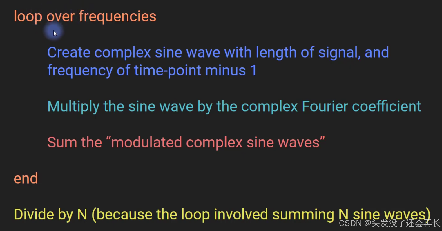
we start off with the Fourier coefficients so we already have all of the complex valued Fourier coefficients and what we want to do is reconstruct a signal in the time domain so here’s how it works you start off with one Fourier coefficient like this so here you see the complex plane and this would be for frequency equals one。 so what you do is you take this Fourier coefficient and you multiply it by a template complex sine wave. because it doesn’t have its own unique amplitude or phase parameter so the amplitude is 1 and the phase is set to zero.
next step is to take another Fourier coefficient at a different frequency and multiply taht by another complex sine wave and of course the frequency of this complex sine wave corresponds to the frequency from which you took this Fourier coefficient. from 1 to n then you simply sum all of the modulated complex sine waves together so you sum all of these things
why we need forward/ inverse FT?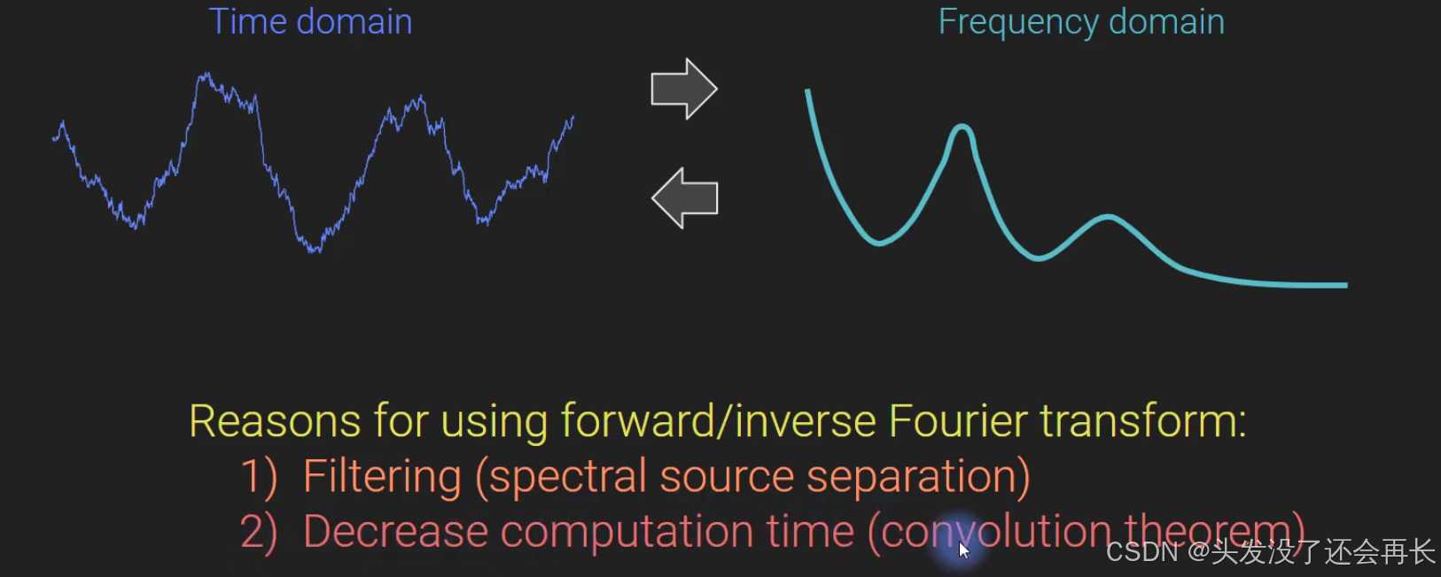
Frequency resolution and zero-padding
the number of frequencies the number of sine waves that we construct in the Fourier transform is a product of N or is determined by n where n is the length of the signal this is the number of time points you have in your signal.
so here we have a short signal with only a few time points and that means we have pretty sparse frequency sampling here.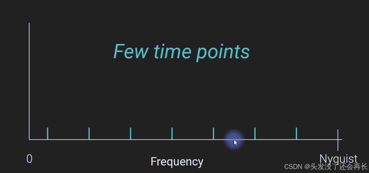
now imagine what happens if we take more time points from that same signal so we just take a longer data segment well M is now higher so zero hasn’t changed the Nyquist frequency hasn’t changed because we still have the same sampling rate but we have more points between zero and Nyquist so the frequency resolution is higher.
we have this is a technical term here buckets of time points. so is the frequency resolution is determined by the number of time points.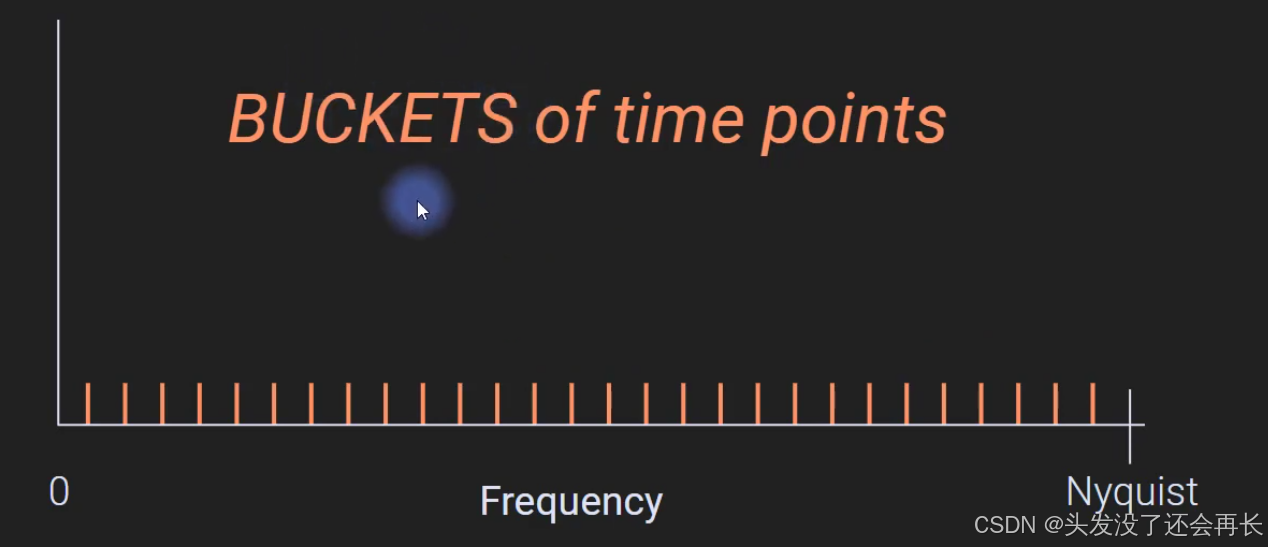
longer segments what you can do is a procedure called zero padding so as you might guess from the name what we do in zero padding is pad the signal with zeros so that looks like this here is our original signal it’s just a little hill but this is the original signal and what I’ve done here is zero pad so I’ve added a bunch of zeros to the end of the signal so here the signal is 20 points long here the signal is 40 points long so now it has twice as many points and that means that when we take the Fourier transform of this this signal it’s going to have twice the frequency resolution as original signal.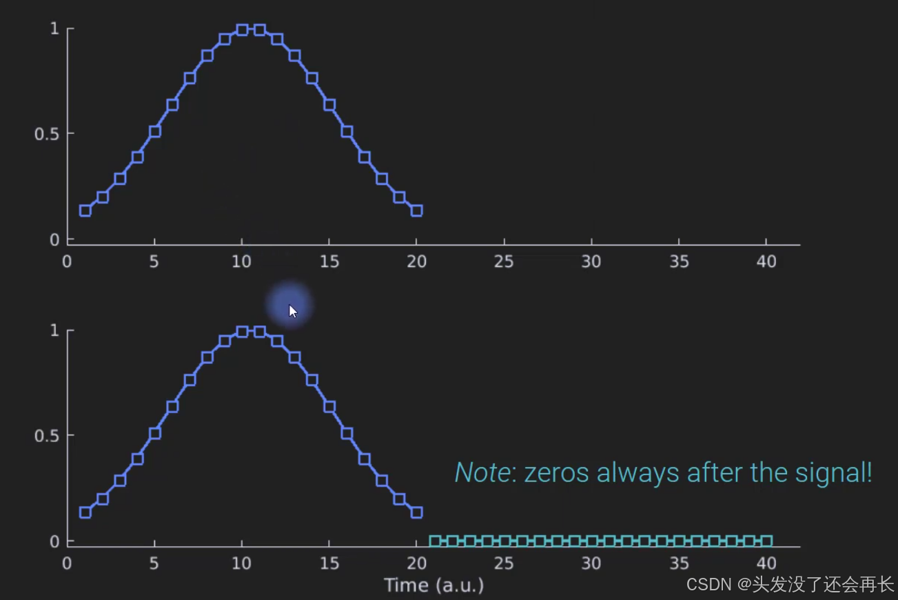
zero padding your signal in practical data analysis there are in fact three motivations for zero padding.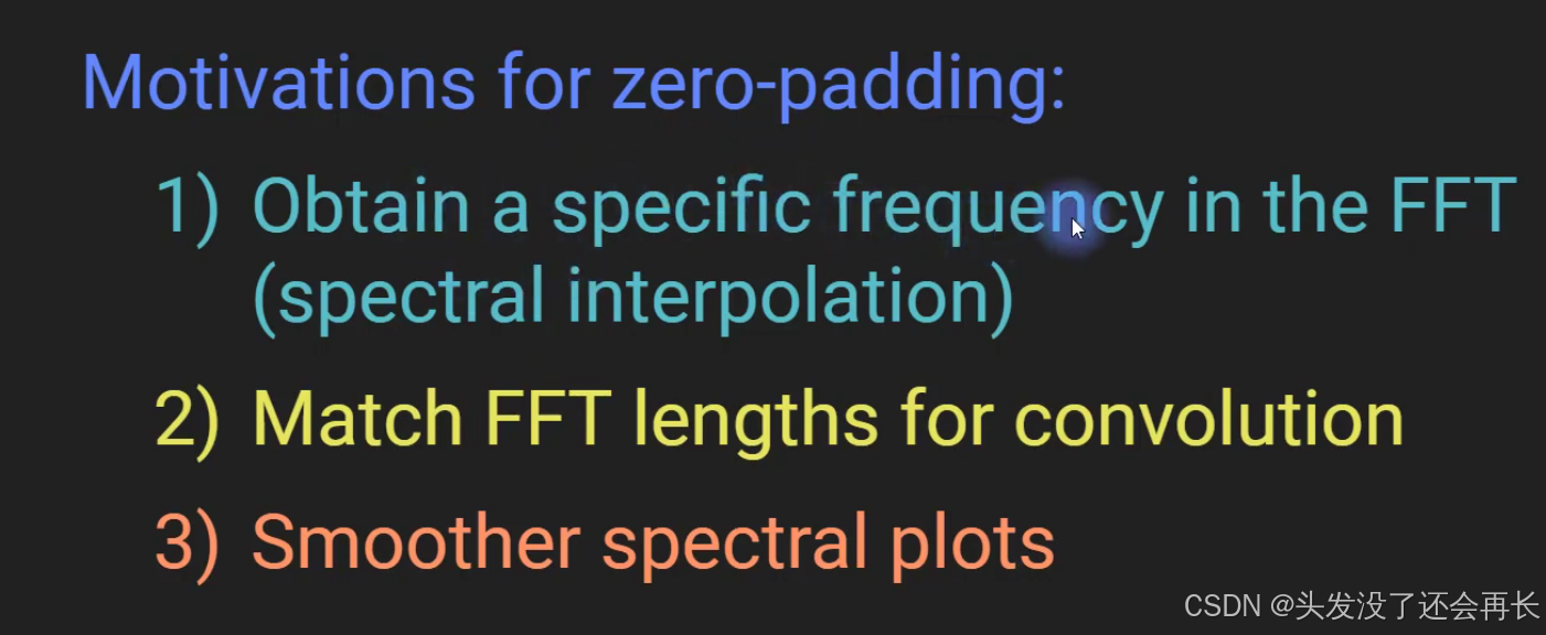
Estimation errors and Fourier coefficients
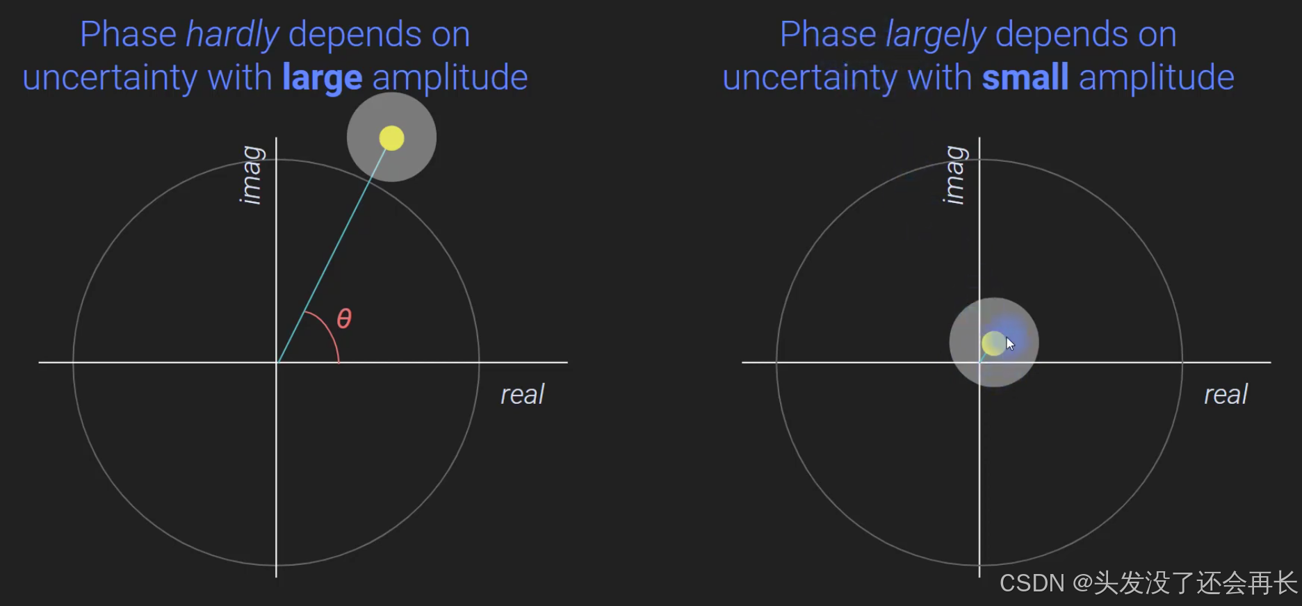
you saw that we can have a sine wave with an amplitude parameter that is independent of the phase so the phase here is of course as you know this angle relative to the positive real axis of the line that connects the origin to the complex Fourier coefficient.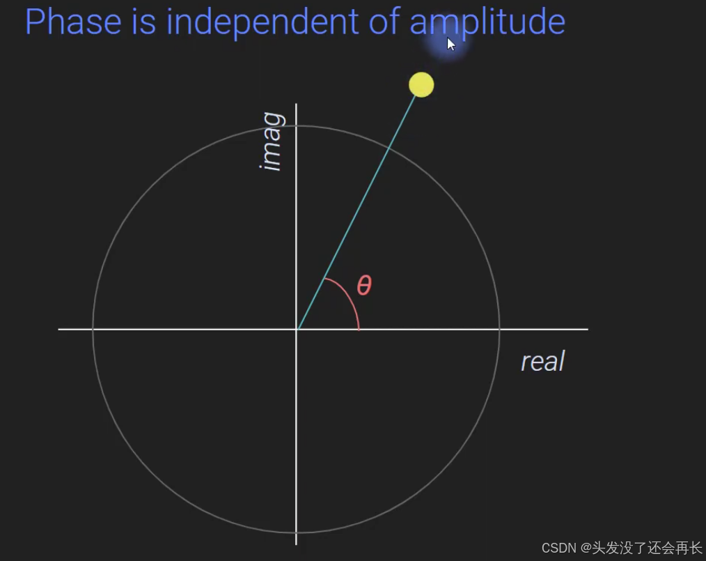
made what is the one case where the phase is not independent of amplitude where you change the amplitude of this coefficient is when the amplitude is exactly zero so when there is zero amplitude or zero power then this Fourier coefficient lies exactly at the origin of this plane and what is the phase for a vector that has no length well I mean it’s undefined.
course in the context of the Fourier transform an amplitude of zero for some Fourier coefficient means that the signal has no energy.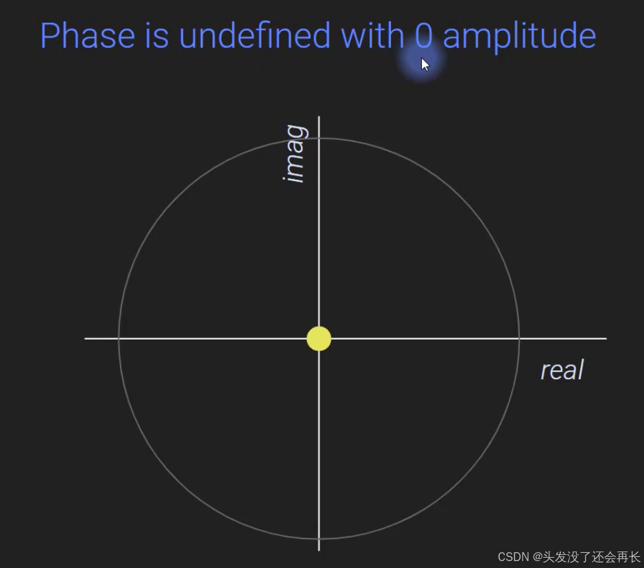
let’s say hundred times so you repeat the the data a hundred times you get a hundred different Fourier coefficients one for each stimulus ret presentation and then you can plot all of those Fourier coefficients and estimate their uncertainty and maybe that cloud of uncertainty looks something like this and this point here is the average of all of those hundred repetitions so essentially what that means is that the true underlying Fourier coefficient.
when amplitude is large we confident that the value we estimate for phase in the real signal is is pretty accurate and when the amplitude is small then we can be less confident we don’t have a lot of confidence in our estimate of phase.