
阅读量:4
前言
最近博主正在和队友准备九月的数学建模,在做往年的题目,博主主要是负责数据处理,运算以及可视化,这里分享一下自己部分的工作,相关题目以及下面所涉及的代码后续我会作为资源上传
问题求解
第一题
第一题的思路主要如下: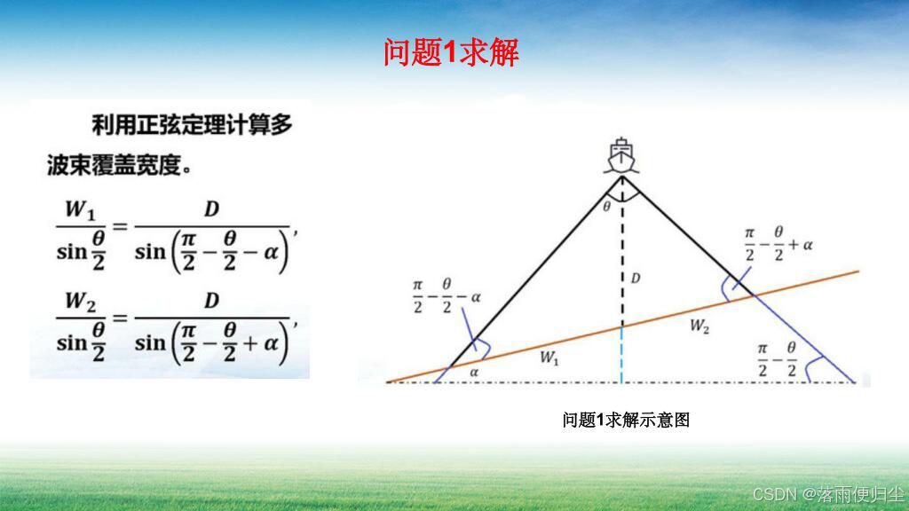
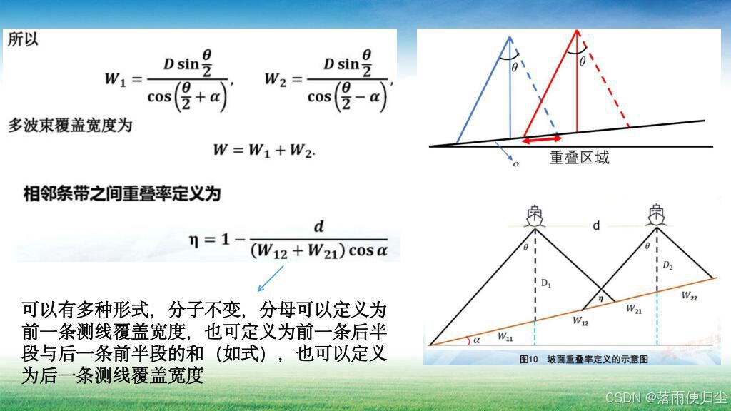
如果我们基于代码实现的话,代码应该是这样的:
# 导入相关第三方包 import numpy as np import pandas as pd import matplotlib.pyplot as plt import math # 生成测线距离中心点处的距离 list1=[] d=200 for i in range(-800,1000,200): list1.append(i) df=pd.DataFrame(list1,columns=["测线距离中心点处的距离"]) #计算海水深度和覆盖宽度 degree1 = 1.5 radian1 = degree1 * (math.pi / 180) df["海水深度"]=(70-df["测线距离中心点处的距离"]*math.tan(radian1)) df["海水深度"]=df["海水深度"].round(2) degrees2 = 120/2 radian2 = degrees2 * (math.pi / 180) df["覆盖宽度"]=(df["海水深度"]*math.sin(radian2)/math.cos(radian2+radian1))+(df["海水深度"]*math.sin(radian2)/math.cos(radian2-radian1)) df["覆盖宽度"]=df["覆盖宽度"].round(2) # 计算重叠率 leftlist=df["海水深度"]*math.sin(radian2)*1/math.cos(radian1+radian2) rightlist=df["海水深度"]*math.sin(radian2)*1/math.cos(radian1-radian2) leftlist=leftlist.round(2) rightlist=rightlist.round(2) leftlist=leftlist.tolist() leftlist=leftlist[1:] rightlist=rightlist.tolist() rightlist=rightlist[:8] heights = df["覆盖宽度"].tolist() heights=heights[:8] list2=[0] for i in range(0,8): a=(1-200/((leftlist[i]+rightlist[i])*math.cos(radian1))) list2.append(a*100) df["重叠率"]=list2 df.to_excel("2023B题1.xlsx",index=False) 这样我们就基本上完成了对相关数据的求解,然后我们可以实现一下对于它的可视化,代码与相关结果如下:
plt.rcParams['font.sans-serif'] = ['SimHei'] # 指定默认字体 plt.rcParams['axes.unicode_minus'] = False # 解决保存图像是负号'-'显示为方块的问题 # Plotting sea depth plt.figure(figsize=(10, 6)) plt.plot(df["测线距离中心点处的距离"], df["海水深度"], marker='o', linestyle='-', color='b', label='海水深度') # Plotting coverage width plt.plot(df["测线距离中心点处的距离"], df["覆盖宽度"], marker='o', linestyle='-', color='g', label='覆盖宽度') # Plotting overlap rate plt.plot(df["测线距离中心点处的距离"], df["重叠率"], marker='o', linestyle='-', color='r', label='重叠率') # Adding labels and title plt.xlabel('测线距离中心点处的距离') plt.ylabel('海水深度 / 覆盖宽度 / 重叠率') plt.title('海水深度、覆盖宽度和重叠率随距离变化的折线图') plt.legend() # Display plot plt.grid(True) plt.tight_layout() plt.show() 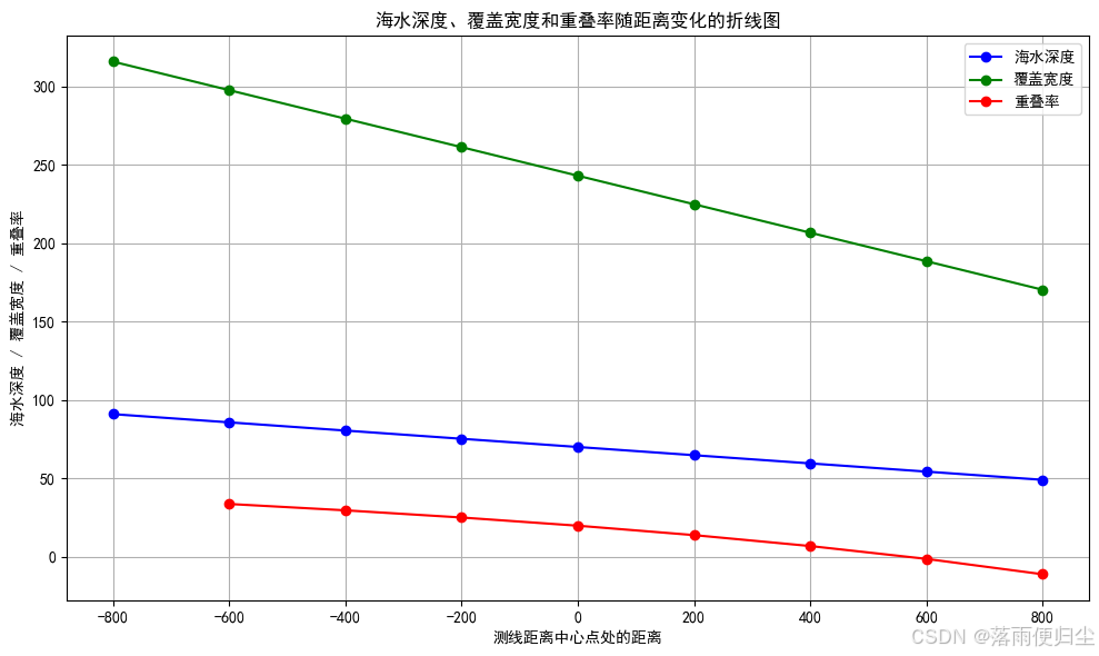
第二题
第二题的思路主要是下面的式子: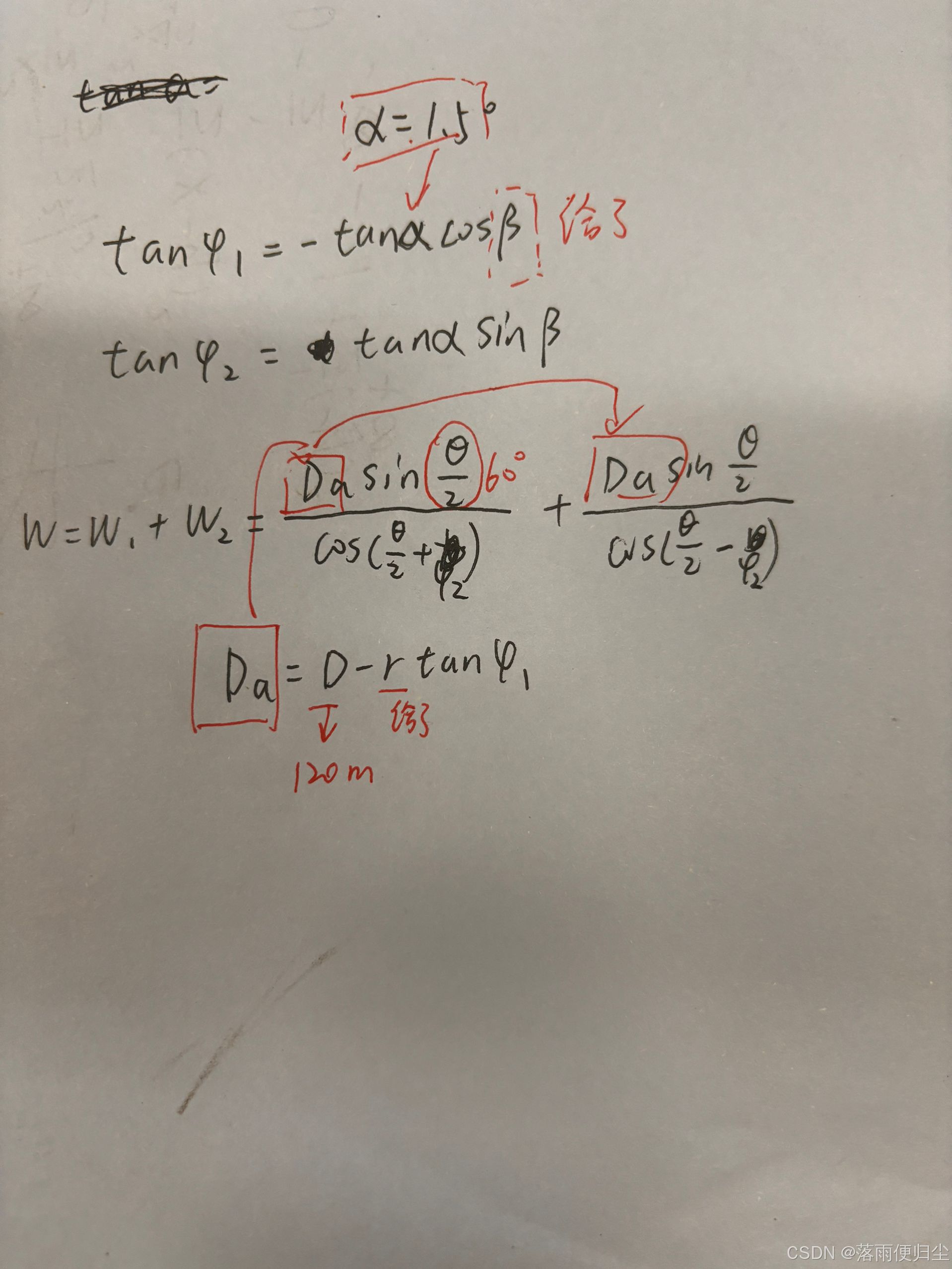
博主的求解代码基本如下:
import numpy as np import pandas as pd import matplotlib.pyplot as plt import math # 生成相关数据 list1=[] list2=[] a=0 for i in range(8): ans=a*math.pi/180 list1.append(ans) a+=45 a=0 for i in range(8): list2.append(a) a+=0.3 b=1.5 c=60 randian11=b*math.pi/180 randian12=c*math.pi/180 # 求解覆盖宽度: list3=[] for i in range(8): list4=[] for j in range(8): randian21=math.tan(randian11)*-1*math.cos(list1[i]) randian31=math.tan(randian11)*math.sin(list1[i]) randian22=math.atan(randian21) randian32=math.atan(randian31) Da=120-list2[j]*randian21*1852 W=(Da*math.sin(randian12)/math.cos(randian12+randian32))+(Da*math.sin(randian12)/math.cos(randian12-randian32)) list4.append(W) list3.append(list4) 最后我们的工作就是数据的可视化了,首先是我们的代码部分:
#对结果的可视化 plt.rcParams['font.sans-serif'] = ['SimHei'] # 指定默认字体 plt.rcParams['axes.unicode_minus'] = False # 解决保存图像是负号'-'显示为方块的问题 df=pd.DataFrame() df["β=0°"]=list3[0] df["β=45°"]=list3[1] df["β=90°"]=list3[2] df["β=135°"]=list3[3] df["测量船距海域中心点的距离"]=list2 plt.figure(figsize=(10, 6)) plt.plot(df["测量船距海域中心点的距离"], df["β=0°"], label="β=0°") plt.scatter(df["测量船距海域中心点的距离"], df["β=0°"]) plt.plot(df["测量船距海域中心点的距离"], df["β=45°"], label="β=45°") plt.scatter(df["测量船距海域中心点的距离"], df["β=45°"]) plt.plot(df["测量船距海域中心点的距离"], df["β=90°"], label="β=90°") plt.scatter(df["测量船距海域中心点的距离"], df["β=90°"]) plt.plot(df["测量船距海域中心点的距离"], df["β=135°"], label="β=135°") plt.scatter(df["测量船距海域中心点的距离"], df["β=135°"]) plt.xlabel('测量船距海域中心点的距离') plt.ylabel('list3 values') plt.legend() plt.grid(True) plt.show() 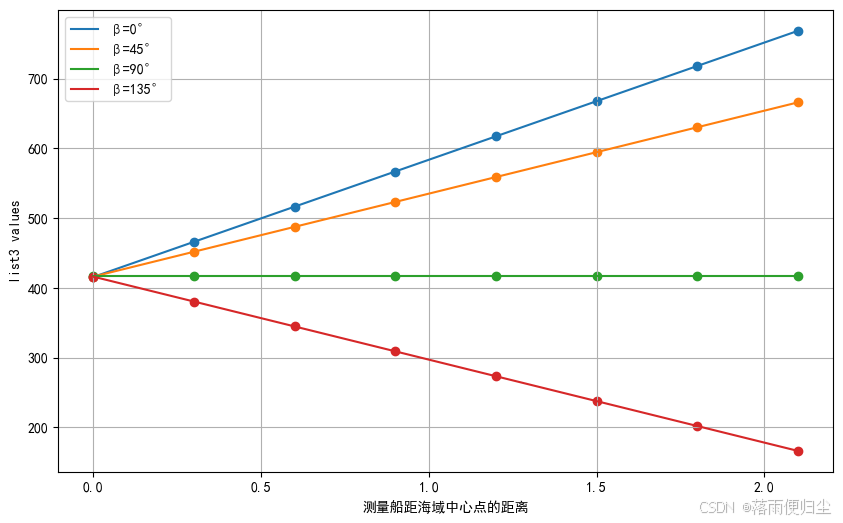
第三题
前言
这题与上面的题目仅仅需要我们求解不同,这题的工作主要分为两份:
- 求解
- 灵敏度分析
求解
这题求解的主要思路如下: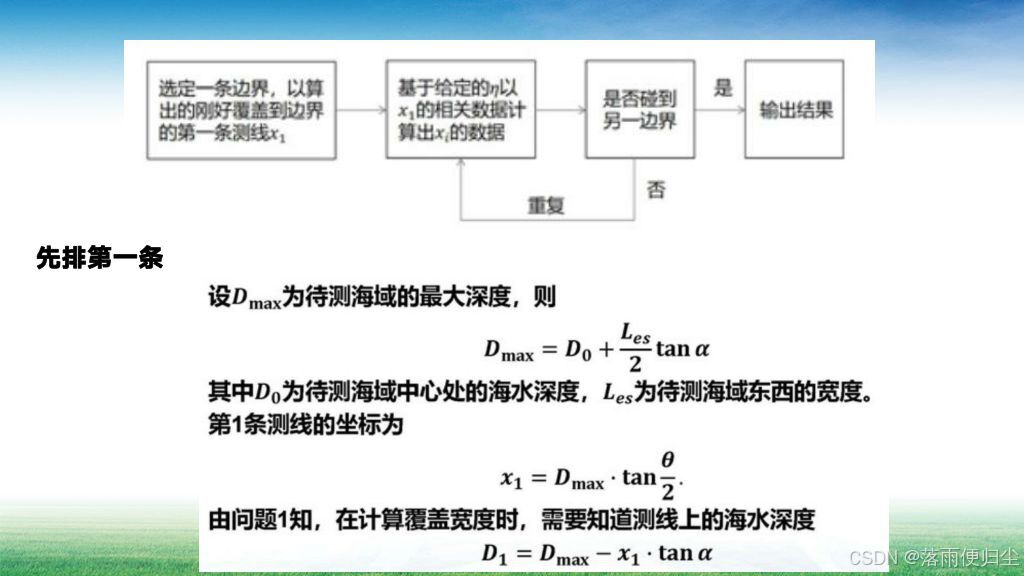
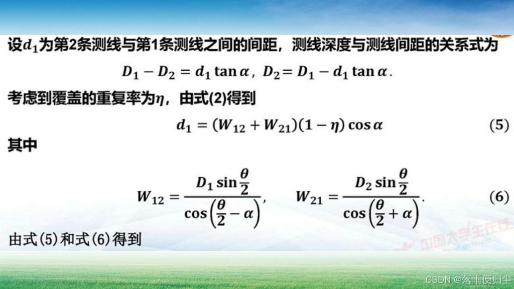
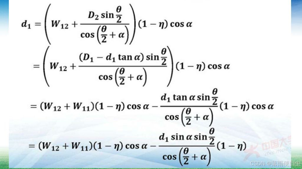
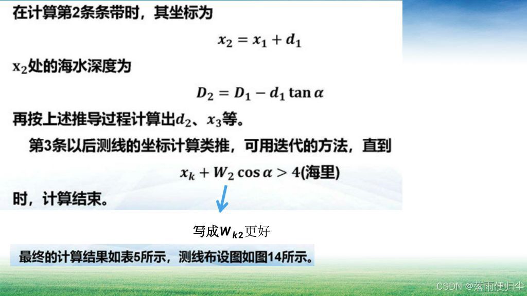
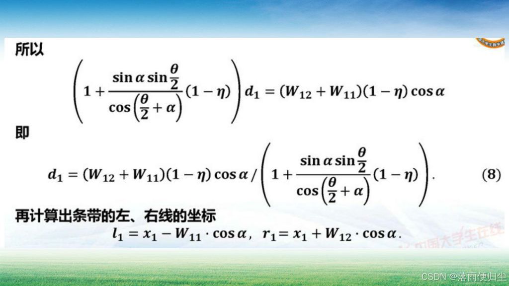
(PS:浅浅吐槽一下,公式真的多,理顺花了我好一会…)
博主的求解代码如下:
import numpy as np import pandas as pd import matplotlib.pyplot as plt import math # 设置相关参数 a=1.5 b=60 radian1=a*math.pi/180 radian2=b* math.pi/180 D0=110 Les=4*1852 #待测海域东西宽度 D=D0+Les/2*math.tan(radian1) #此处Dmax x=D*math.tan(radian2) D=D-x*math.tan(radian1) W1=0 W2=0 res_list=[x] # 存储x left_list=[] # 存储左线坐标 right_list=[] # 存储右线坐标 while x+W2*math.cos(radian1)<=Les: W2=D*math.sin(radian2)/math.cos(radian2-radian1) W1=D*math.sin(radian2)/math.cos(radian2+radian1) d=(W1+W2)*0.9*math.cos(radian1)/(1+math.sin(radian1)*math.sin(radian2)/math.cos(radian2+radian1)*0.9) left_list.append(x-W1*math.cos(radian1)) right_list.append(x+W2*math.cos(radian1)) D=D-d*math.tan(radian1) x=x+d res_list.append(x) W2=D*math.sin(radian2)/math.cos(radian2-radian1) W1=D*math.sin(radian2)/math.cos(radian2+radian1) d=(W1+W2)*0.9*math.cos(radian1)/(1+math.sin(radian1)*math.sin(radian2)/math.cos(radian2+radian1)*0.9) left_list.append(x-W1*math.cos(radian1)) right_list.append(x+W2*math.cos(radian1)) print("总条数:%d"%(len(res_list))) #总条数 print("最大长度:%f"%(res_list[-1])) #最大长度 for i in range(len(res_list)): res_list[i]=res_list[i]/1852 left_list[i]=left_list[i]/1852 right_list[i]=right_list[i]/1852 然后就是我们对相关结果的可视化:
# 可视化 plt.rcParams['font.sans-serif'] = ['SimHei'] # 指定默认字体 plt.rcParams['axes.unicode_minus'] = False # 解决保存图像是负号'-'显示为方块的问题 plt.axvline(res_list[0], color='red',label='Red Line (测线)') plt.axvline(left_list[0], color='green',label='Green Line (条线左侧)') plt.axvline(right_list[0], color='blue',label='Blue Line (条线右侧)') for i in range(1, len(res_list)): plt.axvline(res_list[i], color='red') plt.axvline(left_list[i], color='green') plt.axvline(right_list[i], color='blue') # 设置图形属性 plt.title('问题三结果') plt.ylabel('由南向北/海里') plt.legend() # 显示图形 plt.grid(True) plt.show() 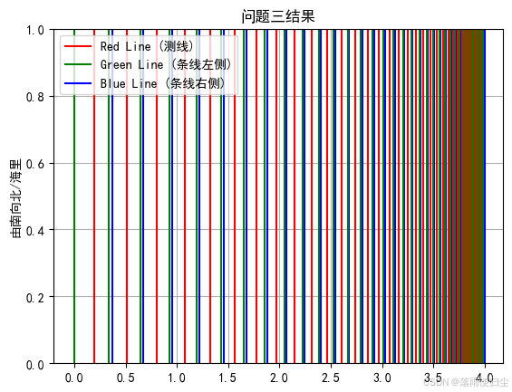
灵敏度分析
灵敏度的分析思路其实还是很简单,主要是我们要改变开角和坡角的大小来看一下
看一下对结果的影响:
基于开角变化实现的灵敏度分析及其可视化
import numpy as np import pandas as pd import matplotlib.pyplot as plt import math # 设置相关参数 for b in range(100,150,10): a=1.5 radian1=a*math.pi/180 radian2=b/2* math.pi/180 D0=110 Les=4*1852 #待测海域东西宽度 D=D0+Les/2*math.tan(radian1) #此处Dmax x=D*math.tan(radian2) D=D-x*math.tan(radian1) W1=0 W2=0 res_list=[x] left_list=[] right_list=[] while x+W2*math.cos(radian1)<=Les: W2=D*math.sin(radian2)/math.cos(radian2-radian1) W1=D*math.sin(radian2)/math.cos(radian2+radian1) d=(W1+W2)*0.9*math.cos(radian1)/(1+math.sin(radian1)*math.sin(radian2)/math.cos(radian2+radian1)*0.9) left_list.append(x-W1*math.cos(radian1)) right_list.append(x+W2*math.cos(radian1)) D=D-d*math.tan(radian1) x=x+d res_list.append(x) W2=D*math.sin(radian2)/math.cos(radian2-radian1) W1=D*math.sin(radian2)/math.cos(radian2+radian1) d=(W1+W2)*0.9*math.cos(radian1)/(1+math.sin(radian1)*math.sin(radian2)/math.cos(radian2+radian1)*0.9) plt.plot(range(len(res_list)), res_list, linestyle='-', label=f'开角为{b}°') plt.rcParams['font.sans-serif'] = ['SimHei'] # 指定默认字体 plt.rcParams['axes.unicode_minus'] = False # 解决保存图像是负号'-'显示为方块的问题 # 设置标签和标题 plt.xlabel('i') plt.ylabel('res_list[i]') plt.title('基于开角变化实现的灵敏度分析及其可视化') # 添加网格线和图例(可选) plt.grid(True) plt.legend() # 显示图形 plt.show() 结果如下: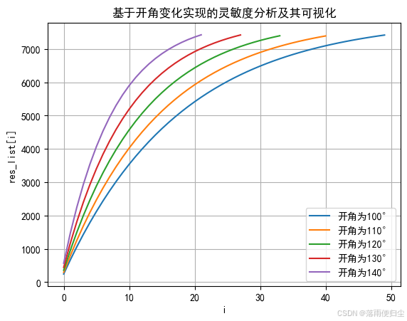
基于开角变化实现的灵敏度分析及其可视化:
import numpy as np import pandas as pd import matplotlib.pyplot as plt import math # 设置相关参数 a_list=[1.3,1.4,1.5] for i in range(len(a_list)): a=a_list[i] b=120 radian1=a*math.pi/180 radian2=b/2* math.pi/180 D0=110 Les=4*1852 #待测海域东西宽度 D=D0+Les/2*math.tan(radian1) #此处Dmax x=D*math.tan(radian2) D=D-x*math.tan(radian1) W1=0 W2=0 res_list=[x] left_list=[] right_list=[] while x+W2*math.cos(radian1)<=Les: W2=D*math.sin(radian2)/math.cos(radian2-radian1) W1=D*math.sin(radian2)/math.cos(radian2+radian1) d=(W1+W2)*0.9*math.cos(radian1)/(1+math.sin(radian1)*math.sin(radian2)/math.cos(radian2+radian1)*0.9) left_list.append(x-W1*math.cos(radian1)) right_list.append(x+W2*math.cos(radian1)) D=D-d*math.tan(radian1) x=x+d res_list.append(x) W2=D*math.sin(radian2)/math.cos(radian2-radian1) W1=D*math.sin(radian2)/math.cos(radian2+radian1) d=(W1+W2)*0.9*math.cos(radian1)/(1+math.sin(radian1)*math.sin(radian2)/math.cos(radian2+radian1)*0.9) plt.plot(range(len(res_list)), res_list, linestyle='-', label=f'坡角为{a}°') plt.rcParams['font.sans-serif'] = ['SimHei'] # 指定默认字体 plt.rcParams['axes.unicode_minus'] = False # 解决保存图像是负号'-'显示为方块的问题 # 设置标签和标题 plt.xlabel('i') plt.ylabel('res_list[i]') plt.title('基于坡角变化实现的灵敏度分析及其可视化') # 添加网格线和图例(可选) plt.grid(True) plt.legend() # 显示图形 plt.show() 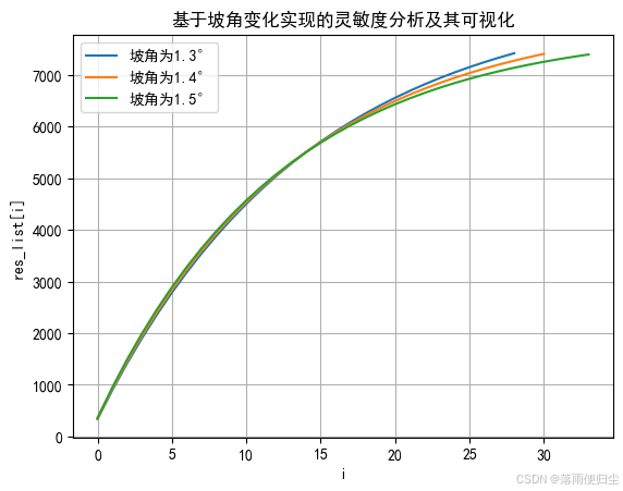
第四题
这题的主要工作就不是我做了,我主要是负责海水深度与横纵坐标数据的可视化,代码如下:
import numpy as np import pandas as pd import matplotlib.pyplot as plt import math # 导入相关数据 filepath="../resource/data.xlsx" df=pd.read_excel(filepath) # 数据预处理 df = df.iloc[1:, 2:] list1=df.values.tolist() list2=[] for i in range(251): list3=[] for j in range(201): list3.append(list1[i][j]*-1) list2.append(list3) list4 = np.arange(0,4.02,0.02) list3 = np.arange(0, 5.02, 0.02) # 数据可视化 plt.rcParams['font.sans-serif'] = ['SimHei'] # 指定默认字体 plt.rcParams['axes.unicode_minus'] = False # 解决保存图像是负号'-'显示为方块的问题 x, y = np.meshgrid(list4, list3) z = np.array(list2) fig = plt.figure(figsize=(10, 8)) ax = fig.add_subplot(111, projection='3d') surf = ax.plot_surface(x, y, z, cmap='viridis') ax.set_xlabel('横向坐标(由西向东)/海里') ax.set_ylabel('纵向坐标(由南向北)/海里') ax.view_init(elev=30, azim=-45) fig.colorbar(surf, aspect=5) # 显示图形 plt.show() 三维图如下: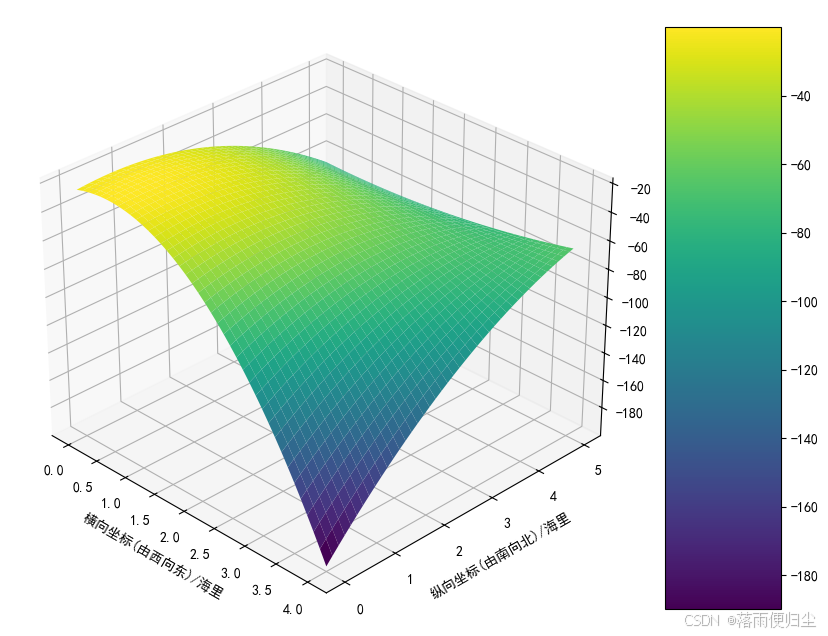
结语
以上就是我所做的所有相关工作了,从这个学期有人找我打一下这个比赛,在此之前我从来都没有写过多少python,前一段时间打数维杯才开始看,没几天就上战场了,所幸最后也水了一个一等奖(感谢我的队友们),之前我的好几个学弟也问过怎么学语言之类,我还是觉得除了我们的第一门语言外,其他的就不要找几十小时的视频看了,你看我没看不也是硬逼出来了吗,事情往往不会在你有充分准备时到来,我们更应该学会边做边学,而不是等到学完再做,种一棵树最好的时间是十年前,其次是现在,写给可能有一些纠结的大家,也写给自己,那我们下篇见!over!
